Page 147 - DECO504_STATISTICAL_METHODS_IN_ECONOMICS_ENGLISH

Unit 9: Correlation: Definition, Types and its Application for Economists

3. A third method of eliminating the long-time tendency and thus isolating the short-time Notes
fluctuations is to assume some curve, represented by an algebraic equation, which “fits” the
statistics in question. The first step in the process is to select some curve, which, for a priori or
other reasons is considered the best representation of the “growth element.”* The second step
is to fit the curve to the statistics; stated algebraically, to determine the constants in the equation
of the curve by use of the actual data. Finally the deviations of the original measurements from
the smooth curve (called by Norton “the growth axis”) are computed. The accuracy with which
one law, the geometric, y = bc , describes the population of the United States, and consequently
x
many things that depend upon population is shown by the following diagram. The full points
are fixed by the actual population according to each of the censuses from 1850. The smooth line
is the graph of the equation
y = 24,086,000 (1.0238) ,
x
which equation was determined from the actual population.
Prof. J. P. Norton has applied the method here described to determine the correlation existing between
percentage of reserves to deposits of New York Associated Banks and call rates.* Weekly statistics
were taken for the period 1885 – 1900. The growth axes assumed were the geometric curve, y = bc ,
x
and the straight line y = a, respectively. (y = the measurement, x = time measured in weeks, while a,
b and c are constants to be determined from the data.) The typical periodic fluctuations of percentage
deviations of reserves and loans were also correlated by this method, using y = bc as the growth
x
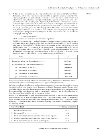
function in both cases. The following table gives the correlation coefficients, ρ .
Series ρ

Reserve deviations and discount rate ................ − 0.37 ± 0.02
(a) Reserve and (b) Loan Periods Immediate..... + 0.49 ± 0.07
(a) precedes (b) by one week .............................. + 0.62 ± 0.06
(a) precedes (b) by two weeks ............................ + 0.87 ± 0.02
(a) precedes (b) by three weeks .......................... + 0.96 ± 0.01

(a) precedes (b) by four weeks ............................ + 0.91 0.05
±
The conclusion from this study is that “the loan period is really the shadow of the reserve period” ...
and apparently follows the latter by “an interval of approximately three weeks.”
Up to this point the problem before us has been the measurement of the amount of correlation between
two variables. This is the simplest case of the general problem of the measurement of the amount of
correlation between one series of measurements, and a group of any number of series of measurements.
The solution of the general problem leads to very complex relations, § and it will not be taken up
here. The case of three variables will be considered briefly.
Messrs. R. H. Hooker and G. U. Yule have considered the problem, To find the relation between the
production of wheat in India during the period 1890 – 1904 (years ending March 31), the price of
wheat (calendar years), and the exports of the subsequent twelve months, 1891 – 1905 (years ending
March 31). The correlation of the annual differences according to the method described in (2) of gives
the following results:
Series Correlated Coefficient Correlation

1. Exports and Production ............... + 0.77
2. Exports and Price .......................... + 0.86
3. Production and Price combined in the ratio 1: 1, and Exports ... + 0.90
4. Production and Price combined in the ratio 3: 1, and Exports ... + 0.81
5. Production and Price in the ratio 1: 3, and Exports ... + 0.58

LOVELY PROFESSIONAL UNIVERSITY 141