Page 296 - DECO504_STATISTICAL_METHODS_IN_ECONOMICS_ENGLISH

Unit 22: Time Series Analysis—Introduction and Components of Time Series

Notes
1979 I 7.5 6.82 111.0
II 6.9 6.90 100.0
III 7.3 6.98 104.6
IV 7.5 7.06 106.2
The irregular variation is assumed to be short-term and relatively insignificant. We have, thus,
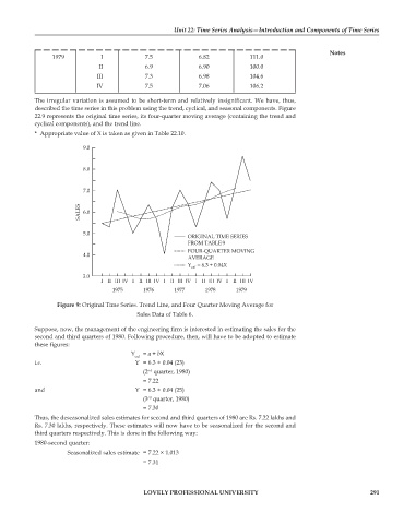
described the time series in this problem using the trend, cyclical, and seasonal components. Figure
22.9 represents the original time series, its four-quarter moving average (containing the trend and
cyclical components), and the trend line.
* Appropriate value of X is taken as given in Table 22.10.

Figure 9: Original Time Series. Trend Line, and Four Quarter Moving Average for
Sales Data of Table 6.

Suppose, now, the management of the engineering firm is interested in estimating the sales for the
second and third quarters of 1980. Following procedure, then, will have to be adopted to estimate
these figures:
Y = a + bX
cal
i.e. Y = 6.3 + 0.04 (23)
(2 quarter, 1980)
nd
= 7.22
and Y = 6.3 + 0.04 (25)
(3 quarter, 1980)
rd
= 7.30
Thus, the deseasonalized sales estimates for second and third quarters of 1980 are Rs. 7.22 lakhs and
Rs. 7.30 lakhs, respectively. These estimates will now have to be seasonalized for the second and
third quarters respectively. This is done in the following way:
1980-second quarter:
Seasonalized sales estimate = 7.22 × 1.013
= 7.31

LOVELY PROFESSIONAL UNIVERSITY 291