Page 295 - DECO504_STATISTICAL_METHODS_IN_ECONOMICS_ENGLISH

Statistical Methods in Economics

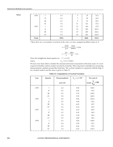
Notes 1978 I 6.5 5 25 32.5

II 6.4 7 49 44.8
III 6.5 9 81 58.5
IV 7.0 11 121 77.0
1979 I 7.5 13 169 97.5
II 6.9 15 225 103.5
III 7.3 17 289 124.1
IV 7.5 19 361 142.5
Total 125.6 2660 114.2

* Since there are even number of periods in the series, we have assigned modified values to X.
∑XY 114.2
b = 2 = = 0.04
∑X 2660.0

∑Y 125.6
a = = = 6.3
n 20
Thus, the straight line trend equation is: Y = a + bX
that is, Y = 6.3 + 0.04 X
cal
We have now been able to identify the seasonal and trend components in the time series. It is now
required to find the cyclical variation around the trend line. This component is identified by measuring
deseasonalized variation around the trend line. The cyclical variation is computed with the help of
the residual method and the same is given in Table 11.
Table 11: Computations of Cyclical Variation

Year Quarter Deseasonalized Y = a + bX* Per cent of
cal
Y
sales (Y) trend Y cal ×100

1975 I 6.9 5.54 124.5
II 5.3 5.62 94.3
III 6.2 5.70 108.8
IV 5.8 5.78 100.3
1976 I 6.0 5.86 102.4
II 5.5 5.94 92.6
III 5.4 6.02 89.7
IV 5.4 6.10 88.5
1977 I 5.0 6.18 80.9
II 6.2 6.26 99.0
III 6.0 6.34 94.6
IV 6.3 6.42 98.1
1978 I 6.5 6.50 100.0
II 6.4 6.58 97.3
III 6.5 6.66 97.6
IV 7.0 6.74 103.9

290 LOVELY PROFESSIONAL UNIVERSITY