Page 294 - DECO504_STATISTICAL_METHODS_IN_ECONOMICS_ENGLISH

Unit 22: Time Series Analysis—Introduction and Components of Time Series

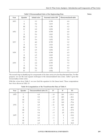
Table 9: Deseasonalized Sales of the Engineering Firm Notes

Year Quarter Actual sales Seasonal index 100 Deseasonalized sales
1975 I 5.5 0.799 6.9
II 5.4 1.013 5.3
III 7.2 1.156 6.2
IV 6.0 1.032 5.8
1976 I 4.8 0.799 6.0
II 5.6 1.013 5.5
III 6.3 1.156 5.4
IV 5.6 1.032 5.4
1977 I 4.0 0.799 5.0
II 6.3 1.013 6.2
III 7.0 1.156 6.0
IV 6.5 1.032 6.3
1978 I 5.2 0.799 6.5
II 6.5 1.013 6.4
III 7.5 1.156 6.5
IV 7.2 1.032 7.0
1979 I 6.0 0.799 7.5
II 7.0 1.013 6.9
III 8.4 1.156 7.3
IV 7.7 1.032 7.5

The second step in identifying the components of the time series is to develop the trend line. For this
purpose, we use the least squares technique to the deseasonalized time series. Table 9 gives the
deseasonalized time series.
With the values from Table 9. we now find the equation for the linear trend. These computations
have been shown in Table 10.

Table 10: Computations of the Trend from the Data of Table 9.
Year Quarter Deseasonalized sales (Y) X* X 2 XY

1975 I 6.9 – 19 361 – 131.1
II 5.3 – 17 289 – 90.1
III 6.2 – 15 225 – 93.0
IV 5.8 – 13 169 – 75.4
1976 I 6.0 – 11 121 – 66.0
II 5.5 – 9 81 – 49.5
III 5.4 – 7 49 – 37.8
IV 5.4 – 5 25 – 27.0
1977 I 5.0 – 3 9 – 15.0
II 6.2 – 1 1 – 6.2
III 6.0 1 1 6.0
IV 6.3 3 9 18.9

LOVELY PROFESSIONAL UNIVERSITY 289