Page 200 - DMTH402_COMPLEX_ANALYSIS_AND_DIFFERENTIAL_GEOMETRY

Unit 17: Tensor Fields in Curvilinear Coordinates

17.8 Differentiation of Tensor Fields in Curvilinear Coordinates Notes

We already know how to differentiate tensor fields in Cartesian coordinates (see section 21). We
know that operator  produces tensor field of type (r, s + 1) when applied to a tensor field of type
(r, s). The only thing we need now is to transform  to a curvilinear coordinate system. In order
to calculate tensor X in curvilinear coordinates, let’s first transform X into auxiliary Cartesian
coordinates, then apply , and then transform X back into curvilinear coordinates:

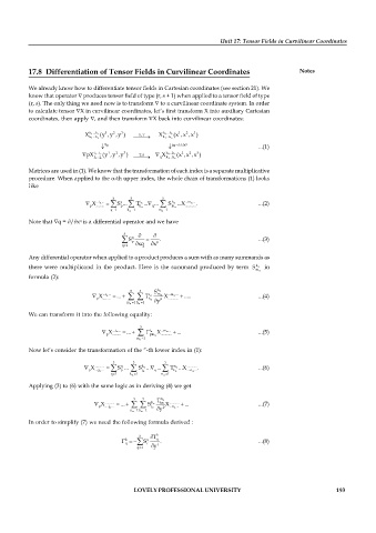
X h k 1 ...h r s (y ,y ,y )  X h k 1 ...h r s (x ,x ,x )
3
2
1
1
2
3
S ,T
1 ...k
1 ...k
/ x
  p   q  q ...(1)
1
2
1 i ...i
3
1
3
2
 pX 1 j ...j r s (y ,y ,y )   q X h k 1 ...h s r (x ,x ,x )
T,S
1 ...k
Matrices are used in (1). We know that the transformation of each index is a separate multiplicative
procedure. When applied to the -th upper index, the whole chain of transformations (1) looks
like
3 3 3
...
...i ...
q
p 
 p X ..........  S ... T ... q  S h  ...X ...m ... . ...(2)

i 


.............
q 1 h   1 h  m   1 m 

Note that q = /x is a differential operator and we have
q
3 q  
 S p  p . ...(3)
q 1  xq x 

Any differential operator when applied to a product produces a sum with as many summands as
there were multiplicand in the product. Here is the summand produced by term S h  in
m 
formula (2):
3 3 S h 
 p X ...i ...  ...    T h  i  m  p X ...m ...  ..... ...(4)


.............
..........
m   1 h   1  y
We can transform it into the following equality:
3
 p X ...i ...  ...    i  X ...m ...  ... ...(5)


.............
..........
m   1 pm 
Now let’s consider the transformation of the ”-th lower index in (1):
3 3 3
...
q
............
p 
 p X ....j ...  S ... S ... q  T ...X ............. . ...(6)

n 
k 
....n ...

q 1 k   1 j  n   1 k  

Applying (3) to (6) with the same logic as in deriving (4) we get
3 3 k T n 
 p X ............  ...    S j   k p X ............  ... ...(7)
....j ...
...n ...

n   1 k   1  y 
In order to simplify (7) we need the following formula derived :
3  T k
k
    S q i q j . ...(8)
ij
q 1  y

LOVELY PROFESSIONAL UNIVERSITY 193