Page 196 - DMTH402_COMPLEX_ANALYSIS_AND_DIFFERENTIAL_GEOMETRY

Unit 17: Tensor Fields in Curvilinear Coordinates

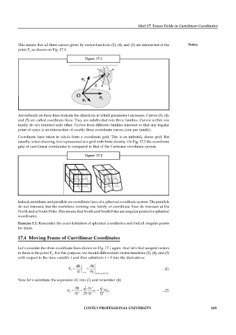
This means that all three curves given by vector-functions (3), (4), and (5) are intersected at the Notes
point P as shown on Fig. 17.1.
0
Figure 17.1

Arrowheads on these lines indicate the directions in which parameter t increases. Curves (3), (4),
and (5) are called coordinate lines. They are subdivided into three families. Curves within one
family do not intersect each other. Curves from different families intersect so that any regular
point of space is an intersection of exactly three coordinate curves (one per family).
Coordinate lines taken in whole form a coordinate grid. This is an infinitely dense grid. But
usually, when drawing, it is represented as a grid with finite density. On Fig. 17.2 the coordinate
grid of curvilinear coordinates is compared to that of the Cartesian coordinate system.

Figure 17.2

Indeed, meridians and parallels are coordinate lines of a spherical coordinate system. The parallels
do not intersect, but the meridians forming one family of coordinate lines do intersect at the
North and at South Poles. This means that North and South Poles are singular points for spherical
coordinates.
Exercise 1.1: Remember the exact definition of spherical coordinates and find all singular points
for them.

17.4 Moving Frame of Curvilinear Coordinates

Let’s consider the three coordinate lines shown on Fig. 17.1 again. And let’s find tangent vectors
to them at the point P . For this purpose, we should differentiate vector-functions (3), (4), and (5)
0
with respect to the time variable t and then substitute t = 0 into the derivatives:
dR  R
E  dt i t 0   y i at the point 0 P . ...(1)
i

Now let’s substitute the expansion (1) into (1) and remember (4):

 R 3  x j 3 j
j 
E  i  e  S e . j ...(2)

i
i
 y j 1 y i j 1


LOVELY PROFESSIONAL UNIVERSITY 189