Page 159 - DMTH404_STATISTICS

Unit 11: Chebyshev’s Inequality

2
Theorem 1: Suppose X is a random variable with mean  and finite variance  . Then for every Notes
 > 0.
Proof: We shall prove the theorem for continuous r.vs. The proof in the discrete case is very
similar.
Suppose X is a random variable with probability density function f. From the definition of the
variance of X, we have
+
 = E [(x – ) ] = (x – ) f(x)dx. 2   2


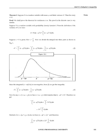
Suppose  > 0 is given. Put   . Now we divide the integral into three parts as shown in
1

Fig. 1.
 1   1  
2
2
2
2
   (x   ) f(x)dx   (x   ) f(x)dx   (x   ) f(x)dx ...(2)
  1   1 
Figure 11.1

Since the integrand (x – m)2 f(x) is non-negative, from (2) we get the inequality
 1  
2
2
2
   (x   ) f(x)dx   (x   ) f(x)dx ...(3)
  1 
2
2
2
Now for any x  ]–,  –  ], we have x   –   which implies that (x – )    . Therefore we
1 1
get
 1   1 
2
2
 (x   ) f(x)dx     2 f(x)dx
 
 1 
2
=   2  f(x)dx.

2
2
2
Similarly for x  ] +  , [ also we have (x – )    and therefore
1 1
 
2
2
 (x   ) f(x)dx    2  f(x)dx
1
 1   1 
LOVELY PROFESSIONAL UNIVERSITY 151