Page 160 - DMTH404_STATISTICS

Statistics

Notes Then by (3) we get

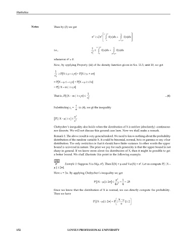
  1   
2
2
2
      f(x)dx   f(x)dx
1
    1   
 1  
1
i.e.,   f(x)dx   f(x)dx
 2
1   1 
2
whenever   0.
Now, by applying Property (iii) of the density function given in Sec. 11.3, unit 10, we get
1
 P[X   –  ] + P[X   + ]
 2 1
1
= P[X –   –  ] + P[X –   1]
1
= P[|X – m|   ]
1
1
That is, P[|X – m|   ]  ...(4)
1  2
1

Substituting  = in (4), we gt the inequality
1 

 2
P[|X   |   
 2
Chebyshev’s inequality also holds when the distribution of X is neither (absolutely) continuous
nor discrete. We will not discuss this general case here. Now we shall make a remark.
Remark 1: The above result is very general indeed. We need to know nothing about the probability
distribution of the random variable X. It could be binomial, normal, beta or gamma or any other
distribution. The only restriction is that it should have finite variance. In other words the upper
bound is universal in nature. The price we pay for such generality is that the upper bound is not
sharp in general. If we know more about the distribution of X, then it might be possible to get
a better bound. We shall illustrate this point in the following example.

2
Example 1: Suppose X is N(,  ). Then E(X) =  and Var(X) =  . Let us compute P[ |X –
2
|  2].
Here  = 2. By applying Chebychev’s inequality we get

 2 1

P  |X   | 2     .25
4 2 4
Since we know that the distribution of X is normal, we can directly compute the probability.
Then we have

 X   


P  |X   | 2   P | | 2 

  

152 LOVELY PROFESSIONAL UNIVERSITY