Page 161 - DMTH404_STATISTICS

Unit 11: Chebyshev’s Inequality

Notes
X  
Since has N(0, 1) as its distribution, from the normal distribution table given in the

appendix of Unit 11, we get

 X   
P   2  0.456

  
which is substantially small as compared to the exact value 0.25. Thus in this case we could get
a better upperbound by directly using the distribution.
Let us consider another example.

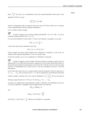
Example 2: Suppose X is a random variable such that P[X = 1] = 1/2 = P[X = –1]. Let us
compute an upper bound for P[|X – |> ].

You can check that E(X) = 0 and Var(X) = 1. Hence, by Chebyshev’s inequality, we get that
 2
P  |X   |     1.
 2
on the other hand, direct calculations show that

P  |X   |   P |X| 1    1.
In this example, the upper bound obtained from Chebyshev’s inequality as well as the one
obtained from using the distribution of X are one and the same.
In the first example you can see an application of Chebyshev’s inequality.

Example 3: Suppose a person makes 100 check transactions during a certain period. In
balancing his or her check book transactions, suppose he or she rounds off the check entries to
the nearest rupee instead of subtracting the exact amount he or she has used. Let us find an upper
bound to the probability that the total error he or she has committed exceeds Rs. 5 after 100
transactions.
Let X denote the round off error in rupees made for the ith transaction. Then the total error is
i
X + X + ..... + X . We can assume that X , 1  i  100 are independent and idelltically distributed
1 2 100 i
 1 1 
random variables and that each X has uniform distribution on  , . We are interested in
i  
 2 2 
P
finding an upper bound for the  |S 100 |  5 where S = X + ..... + X .
100
100
1
In general, it is difficult and computationally complex to find the exact distribution. However,
we can use Chebyshev’s inequality to get an upper hound. It is clear that
E(S ) = 100E(X ) = 0
100 1
and
100
var(S ) = 100 var (X ) = .
100 i 12

1
since E(X ) = 0 and Var(X ) = . Therefore by Chebyshev’s inequality,
1 1 12

LOVELY PROFESSIONAL UNIVERSITY 153