Page 225 - DMTH404_STATISTICS

Unit 15: Exponential Distribution and Normal Distribution

Solution. Notes

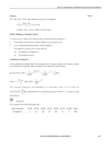
P(X 30) = P(X  29.5) (after making correction for continuity).

-
æ 29.5 25ö
P z= ç  ÷ = P (z  0.9 )
è 5 ø
= 0.5000 – P(0 £ z £ 0.9) = 0.5000 - 0.3159 = 0.1841

15.3.8 Fitting a Normal Curve

A normal curve is fitted to the observed data with the following objectives :
1. To provide a visual device to judge whether it is a good fit or not.

2. Use to estimate the characteristics of the population.
The fitting of a normal curve can be done by
(a) The Method of Ordinates or

(b) The Method of Areas.
(a) Method of Ordinates

In this method, the ordinate f(X) of the normal curve, for various values of the random variate
X are obtained by using the table of ordinates for a standard normal variate.

-
æ
1 X m ö 2 1
1 - ç ÷ 1 - z 2 1
f X
We can write ( ) = e 2 è  ø = e 2 = f ( ) z
 2p  2p 
1
-
X m 1 - z 2
where z = and f ( ) z = e 2 .
 2p
The expected frequency corresponding to a particular value of X is given by
N
y = N . f X f ( ) z and therefore, the expected frequency of a class = y ´ h, where h is the
( ) =

class interval.

Example 41:
Fit a normal curve to the following data :

Class Intervals : 10-20 20-30 30-40 40-50 50-60 60-70 70-80 Total
Frequency : 2 11 24 33 20 8 2 100

LOVELY PROFESSIONAL UNIVERSITY 217