Page 226 - DMTH404_STATISTICS

Statistics

Notes Solution.

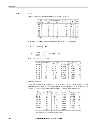
First we compute mean and standard deviation of the given data.

Class Mid - values Frequency X - 45 2
d = fd fd
Intervals (X) ( f ) 10
10 - 20 15 2 - 3 - 6 18
20 - 30 25 11 - 2 - 22 44
30 - 40 35 24 - 1 - 24 24
40 - 50 45 33 0 0 0
50 - 60 55 20 1 20 20
60 -70 65 8 2 16 32
70 - 80 75 2 3 6 18
Total 100 - 10 156

Note: If the class intervals are not continuous, they should first be made so.

10
-
 m = 45 10 ´ = 44
100

2
156 æ 10 ö
and  = 10 - ç ÷ = 10 1.55 = 12.4
100 è 100 ø
Table for the fitting of Normal Curve
X - m f z a f
Class Mid - values z = y = N
Intervals (X) s ( from table) s f z a f f *
e
10 - 20 15 - 2.34 0.0258 0.2081 2
20 - 30 25 - 1.53 0.1238 0.9984 10
30 - 40 35 - 0.73 0.3056 2.4645 25
40 - 50 45 0.08 0.3977 3.2073 32
50 - 60 55 0.89 0.2685 2.1653 22
60 -70 65 1.69 0.0957 0.7718 8
70 - 80 75 2.50 0.0175 0.1411 1

(b) Method of Areas
Under this method, the probabilities or the areas of the random variable lying in various
intervals are determined. These probabilities are then multiplied by N to get the expected
frequencies. This procedure is explained below for the data of the above example.
Class Lower Limit X - 44 Area from Area under
z = f *
Intervals (X) 12.4 0 to z the class e
10 - 20 10 - 2.74 0.4969 0.0231 2
20 - 30 20 - 1.94 0.4738 0.1030 10
30 - 40 30 - 1.13 0.3708 0.2453 25
40 - 50 40 - 0.32 0.1255 0.3099 31
50 - 60 50 0.48 0.1844 0.2171 22
60 -70 60 1.29 0.4015 0.0806 8
70 - 80 70 2.10 0.4821 0.0160 2
80 2.90 0.4981
*Expected frequency approximated to the nearest integer.

218 LOVELY PROFESSIONAL UNIVERSITY