Page 363 - DMTH404_STATISTICS

2
Unit 25: Chi - Sqaure ( ) Distribution

Notes
n 2 n 2
å ( X - X ) å (X - ) m ( X m- ) 2
i
i
=
i 1 i 1 2 2 2
=
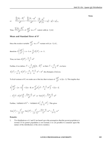
or 2 = 2 - 2 =  -  =  n 1
1
-
n
s s s / n
å ( X - X ) 2 nS 2 2
i
Thus, 2 or 2 is a  -variate with (n - 1) d.f.
s s
Mean and Standard Error of S 2
2
nS  2
Since the random variable 2 is a -variate with (n - 1) d.f.,
s

2
é nS ù n 2
( ) n 1= - .
-
therefore E ê 2 ú = n 1 or 2 E S
ë s û s
n 1 2
-
2
E S
Thus, we have ( ) = s ×
n
1 2 n
2 2 2
Further, if we define s = å ( X - X ) so that s = S × , we have
i
n 1 n 1
-
-
n 2 n n 1 2 2
-
2
( ) =
E s × E S × s × = s (See Remarks 2 below).
( ) =
-
n 1 n 1 n
-
nS 2
2
To find variance of S , we make use of the fact that variance of 2 is 2(n - 1). This implies that
s
2 2
é nS 2 ù n 2 æ 2 n 1 2 ö
-
)
E ê 2 - (n 1- ú = 2 (n 1- ) or 4 E S - s × ÷ = 2 (n 1- )
ç
ë s û s è n ø
( )
2
é
 E S - E S 2 ù 2 = 2 (n 1- ) s × 4 or Var S 2 2 (n 1- ) s × 4
( ) =
ë û n 2 n 2
2
Further, variance of s = variance of æ ç n S × 2 ö ÷ . This gives
è n 1 ø
-
n 2 2 n 2 2 (n 1- ) 4 2 4
2
( ) =
Var s 2 × Var S 2 ´ 2 × s = s ×
( ) =
-
(n 1- ) (n 1- ) n n 1
Remarks:
2
2
1. The distributions of c and S are based upon the assumption that the parent population is
normal. If the parent population is not normal, it is not possible to comment upon the
nature of the distribution of the above statistics.
LOVELY PROFESSIONAL UNIVERSITY 355