Page 361 - DMTH404_STATISTICS

2
Unit 25: Chi - Sqaure ( ) Distribution

Notes
2

25.1 Chi - Square ( ) Distribution
We know that if X is a random variate distributed normally with mean m and standard deviation

-
X m (X m- ) 2
2
s, then z = is a standard normal variate. Square of z, i.e., z = if distributed as
s s 2
2 2
2  
 - variate with one degree of freedom and is written as 1 . Further, the value of 1 , a
squared value, will lie between 0 to , for z lying between -  to . Since most of the z-values are
2 2
close to zero, the probability density of  will be highest near zero. The  distribution with
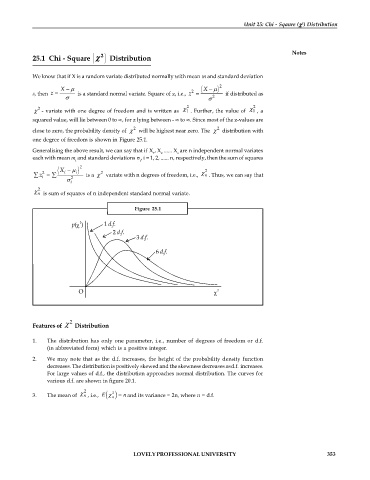
one degree of freedom is shown in Figure 25.1.
Generalising the above result, we can say that if X , X ...... X are n independent normal variates
1 2 n
each with mean m and standard deviations s , i = 1, 2, ...... n, respectively, then the sum of squares
i i
(X - m ) 2 2
2 i i 2 
å z = å 2 is a  variate with n degrees of freedom, i.e., n . Thus, we can say that
i
s i
2
 n is sum of squares of n independent standard normal variate.
Figure 25.1

Features of  2 Distribution

1. The distribution has only one parameter, i.e., number of degrees of freedom or d.f.
(in abbreviated form) which is a positive integer.

2. We may note that as the d.f. increases, the height of the probability density function
decreases. The distribution is positively skewed and the skewness decreases as d.f. increases.
For large values of d.f., the distribution approaches normal distribution. The curves for
various d.f. are shown in figure 20.1.
2
 n , i.e., E  d 2
3. The mean of ni = n and its variance = 2n, where n = d.f.

LOVELY PROFESSIONAL UNIVERSITY 353