Page 73 - DMTH404_STATISTICS

Unit 5: Functions of Random Variables

n Notes
= P [X  z for l  i  n ] –  P[z  X  z ]
1
n
i
i n
i 1

n n
=  P[X  z ]   P[z  X  z ]
i
1
i
n
n


i 1 i 1
n
= [F(z )] – [F(z ) – F(z )] .
n
n n 1
Therefore if –  < z  z < , we get the distribution function as
l n
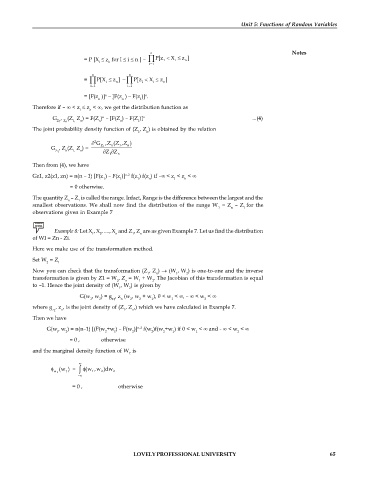
G , (Z Z ) = F(Z ) – [F(Z ) – F(Z )] n ...(4)
n
Z 1 Z n 1, n n n 1
The joint probability density function of (Z , Z ) is obtained by the relation
1 n
 2 G ,Z (Z ,Z )
n
Z
n
1
G , Z (Z Z ) = 1
Z 1 n 1, n  Z Z

1 n
Then from (4), we have
n-2
Gz1, z2(z1, zn) = n(n – 1) [F(z ) – F(z )] f(z ) f(z ) if – < z < z < 
1 1 1 n 1 n
= 0 otherwise.
The quantity Z – Z is called the range. Infact, Range is the difference between the largest and the
n 1
smallest observations. We shall now find the distribution of the range W = Z – Z for the
1 n 1
observations given in Example 7
Example 8: Let X , X , ...., X and Z , Z are as given Example 7. Let us find the distribution
1 2 n 1 n
of WI = Zn - Zi.
Here we make use of the transformation method.
Set W = Z
2 1
Now you can check that the transformation (Z , Z )  (W , W ) is one-to-one and the inverse
1 n 1 2
transformation is given by Z1 = W , Z = W + W . The Jacobian of this transformation is equal
2 n 1 2
to –1. Hence the joint density of (W , W ) is given by
1 2
G(w , w ) = g , z (w , w + w ), 0 < w < , –  < w < 
1 2 z 1 n 2 2 1 1 2
where g , z , is the joint density of (Z , Z ,) which we have calculated in Example 7.
z 1 n 1 n
Then we have
G{w , w ) = n(n–1) [(F(w +w ) – F(w )] f(w )f(w +w ) if 0 < w <  and -  < w < 
n-2
l 2 2 l 2 2 2 1 1 2
= 0 , otherwise
and the marginal density function of W is
1

 w 1 (w ) =   (w ,w )dw 2
1
2
1

= 0 , otherwise

LOVELY PROFESSIONAL UNIVERSITY 65