Page 204 - DMTH505_MEASURE_THEOREY_AND_FUNCTIONAL_ANALYSIS

Unit 16: Continuous Linear Transformations

Notes
1 1
q p
q p
k x k (Using Hölder’s inequality)
k 1 k 1
1
q
q
or |f (x)| k x x  p .
k 1
Hence, we have

1
f(x) q q
sup k = Tf (Using (6))
x 0 x
k 1
which upon using definition of norm yields.

f Tf … (13)
Thus f = Tf (Using (12) and (13))
From the definition of T, it is linear. Also since it is an isometry, it is one-to-one and onto.

*
Hence T is an isometric isomorphism of  onto  , i.e.
p
p
 * 
p q
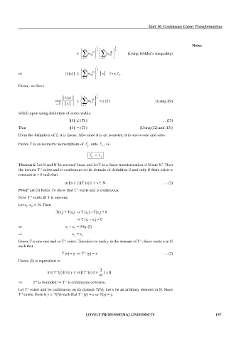
Theorem 6: Let N and N be normed linear and let T be a linear transformation of N into N . Then
–1
the inverse T exists and is continuous on its domain of definition if and only if there exists a
constant m > 0 such that
m x T (x) x N. … (1)
Proof: Let (1) holds. To show that T exists and is continuous.
–1
Now T exists iff T is one-one.
–1
Let x , x , N. Then
1 2
T(x ) = T(x ) T (x ) – T(x ) = 0
1 2 1 2
T (x – x ) = 0
1 2
x – x = 0 by (1)
1 2
x = x
1 2
Hence T is one-one and so T exists. Therefore to each y in the domain of T , there exists x in N
–1
–1
such that
T (x) = y T (y) = x … (2)
–1
Hence (1) is equivalent to
1
–1
–1
m T (y) y T (y) y
m
T is bounded T is continuous converse.
–1
–1
Let T exists and be continuous on its domain T(N). Let x be an arbitrary element in N. Since
–1
–1
–1
T exists, there is y T(N) such that T (y) = x T(x) = y.
LOVELY PROFESSIONAL UNIVERSITY 197