Page 158 - DECO201_MACRO_ECONOMICS_ENGLISH

Unit 9: General Equilibrium of an Economy: IS-LM Analysis

The total demand for money m is then given by Notes
d
m = m + m
d 1 2
or m = kY + h(i)
d
The supply of money m , is determined outside the model and is fixed by the monetary authorities
s
– it is thus exogenous. Thus the supply of money can be written as
m = m
s a
Where, m is simply the amount of money that exists, an amount determined by monetary
a
authorities. Since in equilibrium, demand for money is equal to supply of money, we get the
following three equations to cover the money market.
m = kY + h(i) (demand for money)
d
m = m (supply of money)
s a
m = m (equilibrium condition)
d s
The equilibrium condition ms = m or m = kY + h(i) gives the LM-curve.
d s

Task With the help of a diagram, show the money market equilibrium in a fictitious
economy.
9.3.1 Derivation of LM-curve

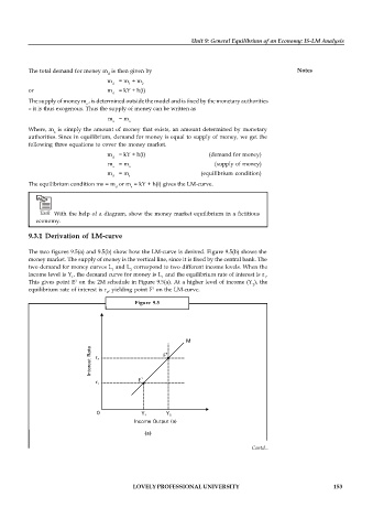
The two figures 9.5(a) and 9.5(b) show how the LM-curve is derived. Figure 9.5(b) shows the
money market. The supply of money is the vertical line, since it is fixed by the central bank. The
two demand for money curves L and L correspond to two different income levels. When the
1 2
income level is Y , the demand curve for money is L and the equilibrium rate of interest is r .
1 1 1
This gives point E on the 2M schedule in Figure 9.5(a). At a higher level of income (Y ), the
1
2
1
equilibrium rate of interest is r , yielding point F on the LM-curve.
2
Figure 9.5

(a)

Contd...

LOVELY PROFESSIONAL UNIVERSITY 153