Page 252 - DMGT209_QUANTITATIVE_TECHNIQUES_II
P. 252

Unit 13: Test of Significance


                                                                                                  Notes
                                   0.1
                               =
                                   0.4
                                  31.62
                                   0.1
                               =        = 8.33
                                  0.012
            As the value of Z at 0.05 =1.64 and calculated value of Z falls in the rejection region, we reject null
            hypothesis, and therefore we conclude that the sale of ‘Femina’ has increased significantly.

            13.2.2  Chi-square Test

            With the help of this test, we will come to know whether two or more attributes are associated
            or not. How much the two attributes are related cannot be by Chi-Square test. Suppose, we have
            certain number of observations classified according to two attributes. We may like to know
            whether a newly introduced medicine is effective in the treatment of certain disease or not.


                !
              Caution   One  case  where  the  distribution  of  the  test  statistic  is  an  exact  chi-square
              distribution is the test that the variance of a normally-distributed population has a given
              value based on a sample variance. Such a test is uncommon in practice because values of
              variances to test against are seldom known exactly.

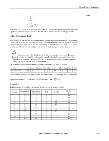
            The numbers of automobile accidents per week in a certain city were as follows:
             Months            Jan   Feb   March   April   May   June   July   Aug   Sep   Oct
             No. of accidents   12   8     20      2    14    10    15    6    9    4

            Does the above data indicate that accident conditions were uniform during the 10- month period.
                                                              100
                                
                                            
                                   
            Expected frequency    12 8 20 2 14 10 15 6 9  4      10
                                                
                                      
                                                      
                                                   
                                         
                                                              10
            Computation
            Null hypothesis: The accident occurrence is uniform over a 10-week period.
                        Observed No.   Expected No.                        O E   2
               Month                               O – E     (O – E) 2
                         of accidents   of accidents                          E
                 1          12           10          2          4            0.4
                 2           8           10         -2          4            0.4
                 3          20           10         10         100           10.0
                 4           2           10         -8         64            6.4
                 5          14           10          4         16            1.6
                 6          10           10          0          0            0.0
                 7          15           10          5         25            2.5
                 8           6           10         -4         16            1.6
                 9           9           10         -1          1            0.1
                 10          4           10         -6         36            3.6
                            100         100          0                       26.6


                                             LOVELY PROFESSIONAL UNIVERSITY                                  247
   247   248   249   250   251   252   253   254   255   256   257