Page 123 - DCOM505_WORKING_CAPITAL_MANAGEMENT

Working Capital Management

Notes with F(A) as the distribution function of A()

E (  h    
r
(  
= - - ( + r   (W * - W 0 + A dF A
W   W 
0  0 W 0 -W * 
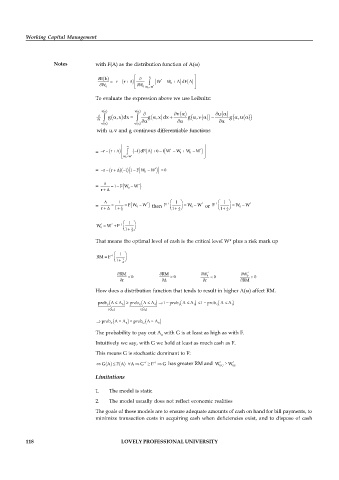
To evaluate the expression above we use Leibnitz:

v (  v ( 

( 
v

d g =  g +   g  u (  g ( 

da  (,x dx   (,x dx  (,v (  -  (,u
u (  u ( 


with u,v and g continous differentiable functions
  
r
= - - ( + r   (  1- dF (  0 1+ -A (W * - W 0 + W 0 - W *  
  W 0 -W *  
= - -r ( + r ( ( 1- 1 - F (W 0 - W *  0=
r
= = 1- ( F W 0 - W * 
r + 
 1 * - 1  1  * - 1  1  *
= = = F (W 0 - W  then F   = W 0 - W or F   = W 0 - W
r
r +  1+ r  1+   1+ 
r
  
 1 
*
W 0 = W * + F - 1  
r
 1+ 

That means the optimal level of cash is the critical level W* plus a risk mark up
 1 
RM  F - 1  
r
 1+ 

RM RM W * W *
< 0  0 0 < 0 0  0
r  r RM
How does a distribution function that tends to result in higher A() affect RM.
prob (A  A  ³ prob ( A A  1- prob ( A A  1 - prob ( A A 
G
F
0
0
  F 0 G 0
( 
( 
F A 0 G A 0
 prob F (A ³ A 0   prob G (A ³ A 0 
The probability to pay out A with G is at least as high as with F.
0
Intuitively we say, with G we hold at least as much cash as F.
This means G is stochastic dominant to F:
*
*
 G (  A F (  A A  G - 1 ³ F - 1  G has greater RM and W 0,G ³ W 0,F
Limitations
1. The model is static

2. The model usually does not reflect economic realities
The goals of these models are to ensure adequate amounts of cash on hand for bill payments, to
minimize transaction costs in acquiring cash when deficiencies exist, and to dispose of cash

118 LOVELY PROFESSIONAL UNIVERSITY