Page 122 - DCOM505_WORKING_CAPITAL_MANAGEMENT

Unit 7: Cash Management

determine the standard deviation of net cash flows the pasty data of the net cash flow behaviour Notes
can be used. Managerial attention is needed only if the cash balance deviates from the limits.

Stone Model

The Stone Model is somewhat similar to the Miller-Orr Model insofar as it uses control limits. It
incorporates, however, a look-ahead forecast of cash flows when an upper or lower limit is hit
to take into account the possibility that the surplus or deficit of cash may naturally correct itself.
If the upper control limit is reached, but is to be followed by cash outflow days that would bring
the cash balance down to an acceptable level, then nothing is done. If instead the surplus cash
would substantially remain that way, then cash is withdrawn to get the cash balance to a
predetermined return point. Of course, if cash were in short supply and the lower control limit
was reached, the opposite would apply. In this way the Stone Model takes into consideration the
cash flow forecast.

Beranek Model

According to Beranek, companies have short-term assets only because they face uncertainties
related to their operations.

Example: A firm could incur substantial costs if the labor force of a vendor supplying a
critical part suddenly went on strike. An inventory of the critical part enables the firm to
continue operating while it seeks an alternate supplier or waits out the strike.

Similarly, a firm may hold a cash reserve to meet unanticipated demand for cash. Since cash is an
unproductive asset, cash reserves are often held in the form of highly liquid short-term
investments.
A = A( the cash out flow depends on the uncertain event w which makes A(w) a stochastic
variable.

W (W ,  = W – A(
1 0 0
Beranek assumes there is a critical cash balance W* which triggers increased cost borrowing
r + . In t = 0 we have cash of W in t = 1  is observed and A() is paid from W (possibly under
0 0
acceptance of penalty interest ). Keep in mind, that W here denotes the cash level that we
0
initially establish in t = 0 with only one cash outflow A() occurring. Where as in Baumol’s
model W denotes the amount that is withdrawn m times.
0
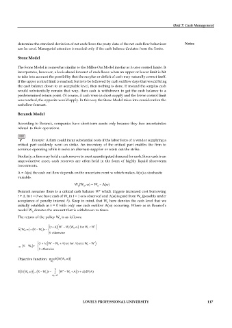
The return of the policy W is as follows:
0
ì ï ( + r ( W * - W (W 0 ,  for W 1 < W * 
h  (W 0  =,  ( -K W r 1
 - í
0
î 0 ï otherwise


ï ( ì + r ( W * - W 0 + A (  for A ( ³ W 0 - W * 
 - í
= ( -K W 0 r
ï î 0 otherwise
Objective function: max E ( (h W , 
0
W 0

( 
E ( (h W 0  =,  ( -K W 0  -r  (W * - W 0 + A ( + r dF A
W 0 -W *

LOVELY PROFESSIONAL UNIVERSITY 117