Page 112 - DCAP601_SIMULATION_AND_MODELING

Simulation and Modelling

Notes 
average queue length =  
1  

 2
= ...(15)
1  
Substituting Eq. (14) into (13), the probability of n customers being in the system can also be
expressed as
n
P =  (1 – ) ...(16)
n
Probability of n customers being in the queue is the same as the probability of (n + 1) customers
being in the system which is
 (1 – ), for n > 0 ...(17)
n+1
Probability of more than n customers being in the system

n
 1   i (1   )

t 0


 1 [(1     (1     2 (1   ) ...   n 1 (1     n (1   )]

)
)
)


 1 [1   n 1 ]

  n 1 ...(18)
These and similar other statistics about the queue are called the operating characteristics of the
queueing system. Derivation of some of the order characteristics are left as exercises. Usually
one is interested in only some of these quantities. As an illustration of how a particular formula
from queueing theory can be put to use, let us consider the following design problem.
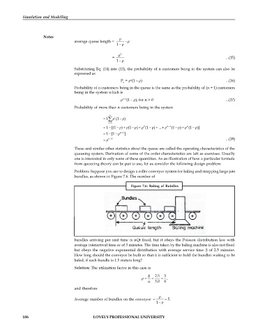
Problem: Suppose you are to design a roller conveyor system for baling and strapping large jute
bundles, as shown in Figure 7.6. The number of
Figure 7.6: Baling of Bubdles

bundles arriving per unit time is nQt fixed, but it obeys the Poisson distribution law with
average interarrival time oc of 3 minutes. The time taken by the baling machine is also not fixed
but obeys the negative exponential distribution with average service time  of 2.5 minutes.
How long should the conveyor be built so that it is sufficient to hold the bundles waiting to be
baled, if each bundle is 1.5 meters long?

Solution: The utilization factor in this case is
 2.5 5
    ,
 3.0 6
and therefore

Average number of bundles on the conveyor   5.
1  

106 LOVELY PROFESSIONAL UNIVERSITY