Page 109 - DCAP601_SIMULATION_AND_MODELING

Unit 7: Simulation of Queuing System (I)

It can be seen that, in general Notes


dq (t) q (t) q (t)
k  k 1 k

dt 
We have already solved this differential equation for k = 1 and 2 (for k = 0, q (t) = f(t)). Solving
o
it successively for k = 3, 4, ... , we will get
k
 t  1
q (t)    e –t / ...(5)
k
   k!
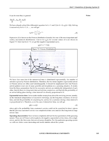
Expression (5) is known as the Poisson distribution formula. It is one of the most important and
widely encountered distributions. Curves for q (t) for several values of k are shown in
k
Figure 7.5. Note that for k = 0, we get the negative exponential curve,
q (t) = e –t/a = f(t)
0
Figure 7.5: Poisson Distribution

We have thus seen that if the interarrival time is distributed exponentially, the number of
arrivals is given by Poisson distribution. Therefore, the two terms negative exponential arrival
or Poisson arrival are often used interchangeably. It should be emphasized here that Poisson
arrival pattern is just one of many possible arrival patterns in a queueing situation. It results
from the three assumptions that (i) the successive arrivals are statistically independent of each
other, that (ii) there is a long-term inter-arrival time constant ex, and that (iii) the probability of
an arrival taking place during a time interval h is directly proportional to h.

Exponential service time: Let us make similar assumptions about the servicing process, namely,
(i) the statistical independence of successive servicings, (ii) the long-term constancy of service
time, and (iii) the probability of completing the .service for a customer during a time interval h
is proportional to h. Therefore, as in the case of interarrival time, we will get
g(t) = e–t/ ...(6)

where g(t) is the probability that a customer's service could not be completed in time t, (given
that the previous customer's service was completed at time zero) and  is the long-term average
service time.
Operating characteristics: Now we have completely defined the four parameters of the queueing
system. These are (i) Poisson arrival pattern, (ii) negative exponential service times, (iii) a single
server, and (iv) the first-come-first-served queue discipline. For this particular queueing system
we will now derive some interesting and useful statistics about the system:

LOVELY PROFESSIONAL UNIVERSITY 103