Page 108 - DCAP601_SIMULATION_AND_MODELING

Simulation and Modelling

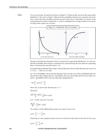
Notes The curves for Eqs. (3) and (4) are shown in Figure 7.4. These are the curves for the exponential
distribution. The curve in Figure 7.4(b) gives the probability that the next customer arrives by
time t, given that the preceding customer arrived at time zero. Customarily the inverse of the
average interarrival time is denoted by , which is nothing but the average number of customers
arriving at the system per unit time.

Figure 7.4 : Interarrival Time of Customers

Having found that the interarrival time is governed by exponential distribution, we will now
find the probability that exactly k customers have arrived during the time interval t (assuming
that no customer had arrived by time t = 0).

Let q (t) be the probability that exactly k arrivals take place between the start time zero and t, for
k
k = I, 2, 3, .... Then we can write
q (t + h) = (Probability that no arrivals take place between time zero and t). (probability that one
l
arrival takes place during time h) + (probability that one arrival takes place between time zero
and t) . (probability that no arrivals take place during time h)

h  h 
 f(t).  q (t). 1  

1
   
where f(t), as previously determined, is e –t/ .
Therefore,


q (t h) q (t) 1
1 1
 [f(t) q (t)]

1
h 
as h  0 this expression becomes
dq (t)  1 [f(t) q (t)]
1

dt  1
The solution of this differential equation can easily be seen to be
1 1
q (t)  e  t /a  f(t)
1
 
Extending the same argument (since at most one arrival can take place in the interval h) we get
2
 t  1
q (t)    .f(t)
2
   2!
102 LOVELY PROFESSIONAL UNIVERSITY