Page 130 - DCAP601_SIMULATION_AND_MODELING

Simulation and Modelling

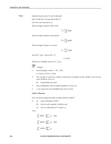
Notes Figures for q(•) and x(•) can be deduced

q(t) = 0 and x(t) = 0 if and only if l(t) = 0
Over the time interval (0, ):
Time-averaged number in the node:

1 
l   l ( )dt
t
 0
Time-averaged number in the queue:
1 
t
q   q ( )dt
 0
Time-averaged number in service:
1 
t
x   x ( )dt
 0
Since l(t) = q(t) + x(t) for all t > 0

x  0.28
Sufficient to calculate any two of , , .l q x

Example
1. From Example 1 (with  = c10 = 376),
l = 1.633 q = 0.710 x = 0.923
2. The average of numerous random observations (samples) of the number in the service
node should be close to l.
(a) Same holds for q and x
3. Server utilization: time-averaged number in service (x)

4. x also represents the probability the server is busy

Little’s Theorem

How are job-averaged and time-average statistics related?
If (a) queue discipline is FIFO,
(b) service node capacity is infinite, and

(c) server is idle both at t = 0 and t = c
n
Then
n c n
t
 l ( )dt   w i and
0 i 1
n c n
 0 q ( )dt   i 1 d i and
t

n c n
 x ( )dt   s i
t
0 i 1

124 LOVELY PROFESSIONAL UNIVERSITY