Page 201 - DCAP601_SIMULATION_AND_MODELING

Unit 11: Design and Evaluation of Simulation Experiments (I)

The key idea is that, if Notes

W and W are the outcomes of two successive simulation runs, then
1 2
 W  W 2  1 1 1
1
Var    Var(W ) Var(W ) Cov(W ,W )].
1
2
1
2
 2  4 4 2
Hence, in the case that W and W are negatively correlated the variance of (W + W )/2 will be
1 2 1 2
smaller than in the case that W and W are independent.
1 2
The question remains how we can achieve that the outcome of two successive simulation runs
will be negatively correlated. From the fact that U and 1 – U are negatively correlated, we may
expect that, if we use the random variables U ,...,U to compute W , the outcome of the first
1 m 1
simulation run, and after that 1 – U ,...,1 – U to compute W , the outcome of the second simulation
1 m 2
run, then also W and W are negatively correlated. Intuition here is that, e.g., in the simulation
1 2
of the G/G/1 queue large realizations of the U 's corresponding to large service times lead to
i
large waiting times in the first run. Using the antithetic variables, this gives small realizations
of the U ' s corresponding to small service times and hence leading to small waiting times in the
i
second run.
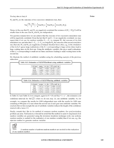
We illustrate the method of antithetic variables using the scheduling example of the previous
subsection.
Table 11.3: Estimation of E(CLPTF)without using antithetic variables

Table 11.4: Estimation of E(CLPTF)using antithetic variables

–x
In Table 11.3 and Table 11.4 we compare, again for N = 10 and F(x) = 1 – e , the estimators and
confidence intervals for E(C LPTF ) when we do not, resp. do, use antithetic variables. So, for
max
example, we compare the results for 1000 independent runs with the results for 1000 runs
consisting of 500 pairs of 2 runs where the second run of each pair uses antithetic variables. We
conclude that in this example the use of antithetic variables reduces the length of the confidence
interval with a factor 1.5.
Finally, remark that, like in the method of common random numbers, the synchronization
problem can arise. Furthermore, it should be noted that the method is easier to implement if all
random variables are generated using the inversion transform technique (only one uniform
random number is needed for the realization of one random variable) than if we use, e.g., the
rejection method to generate random variables

Notes A random number of uniform random numbers are needed for the realization
of one random number.

LOVELY PROFESSIONAL UNIVERSITY 195