Page 72 - DMGT206_PRODUCTION_AND_OPERATIONS_MANAGEMENT
P. 72
Unit 4: Quality Control


          The common approach to on-line quality control is straightforward: We simply take out samples  Notes
          of a definite size from the ongoing production process. We afterward produce line charts of the
          variability in those samples and think about their closeness to target specifications. If a trend
          comes into view in those  lines, or if samples fall outside pre-specified limits,  we state  the
          process to be out of control and take action to locate the cause of the problem. These types of
          charts are at times also referred to as Shewhart control charts named after W. A. Shewhart, who
          is usually credited as being the first to initiate these methods.

          Short Run Control Charts

          The short run control chart, or else control chart for short production runs, plots interpretation
          of  variables or  attributes for several parts on the same chart.  Short run control charts were
          developed to deal with the requirement that several dozen measurements of a process have to
          be collected before control limits are calculated. Meeting this requirement is habitually difficult
          for operations that produce a limited number of an exacting part during a production run.


                 Example: A paper mill may produce only three or four (huge) rolls of a particular kind
          of paper (i.e., part) and then shift production to another kind of paper. But if variables, such as
          paper thickness, or attributes, such as blemishes, are monitored for several dozen rolls of paper
          of, say, a dozen different kinds, control limits for thickness and blemishes could be calculated
          for the transformed (within the short production run) variable values of interest.

          4.2.2  Control Limits

          We are aware from our basic statistics course that plus and minus three standard deviations
          from the mean of normal destruction will include 99.73 per cent of all data in the distribution.
          When the mean absolute deviation of a data set is  less than three standard  deviations, it  is
          considered to be within acceptable limits or error. Using the same rationale, the Upper Control
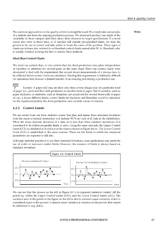
          Limit (UCL) is calculated as 3s and set on the chart as shown in Figure below. The Lower Control
          Limit (LCL) is established in the same manner. These are the limits in which the measured
          parameters are expected to fall into.

          Although, industry practice is to use three standard deviations, some applications may merit the
          use of wider or narrower control limits. However, the measure of limits is always based on
          standard deviations.

                                      Figure  4.1: Control  Charts

                Process in Statistical Control
                                                       Process Out of Statistical Control

           UCL                                     UCL
            CL
                                                    CL
           LCL
                                                   LCL
                                              Time                                Time

          We can see that the process on the left in Figure 4.1 is in apparent statistical control. All the
          points lay within the Upper Control Limits (UCL) and the Lower Control Limits (LCL). The
          variation seen in the points in the figure on the left is due to common cause variation, which is
          considered a part of the process. Common cause variation is variation in the process that cannot
          be attributed to any defect.


                                           LOVELY PROFESSIONAL UNIVERSITY                                   67

