Page 246 - DMGT403_ACCOUNTING_FOR_MANAGERS

Unit 11: Variance Analysis

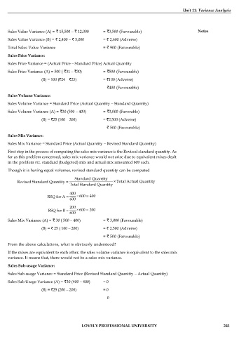
Sales Value Variance (A) = 15,500 – 12,000 = 3,500 (Favourable) Notes
Sales Value Variance (B) = 2,400 – 5,000 = 2,600 (Adverse)
Total Sales Value Variance = 900 (Favourable)
Sales Price Variance:

Sales Price Variance = (Actual Price – Standard Price) Actual Quantity
Sales Price Variance (A) = 500 ( 31 – 30) = 500 (Favourable)
(B) = 100 ( 24 – 25) = 100 (Adverse)
= 400 (Favourable)

Sales Volume Variance:
Sales Volume Variance = Standard Price (Actual Quantity – Standard Quantity)
Sales Volume Variance (A) = 30 (500 – 400) = 3,000 (Favorable)
(B) = 25 (100 – 200) = 2,500 (Adverse)

= 500 (Favourable)
Sales Mix Variance:
Sales Mix Variance = Standard Price (Actual Quantity – Revised Standard Quantity)
First step in the process of computing the sales mix variance is the Revised standard quantity. As
far as this problem concerned, sales mix variance would not arise due to equivalent mixes dealt
in the problem viz. standard (budgeted) mix and actual mix amounted 600 each.

Though it is having equal volumes, revised standard quantity can be computed
Standard Quantity
Revised Standard Quantity = × Total Actual Quantity
Total Standard Quantity
400
RSQ for A = ×600 400
600
200
RSQ for B = ×600 200
600
Sales Mix Variance (A) = 30 ( 500 – 400) = 3,000 (Favourable)
(B) = 25 ( 100 – 200) = 2,500 (Adverse)
= 500 (Favourable)

From the above calculations, what is obviously understood?
If the mixes are equivalent to each other, the sales volume variance is equivalent to the sales mix
variance. It means that, there would not be a sales mix variance.

Sales Sub-usage Variance:
Sales Sub-usage Variance = Standard Price (Revised Standard Quantity – Actual Quantity)
Sales Sub Usage Variance (A) = 30 (400 – 400) = 0
(B) = 25 (200 – 200) = 0
0

LOVELY PROFESSIONAL UNIVERSITY 241