Page 199 - DMGT404 RESEARCH_METHODOLOGY

Unit 9: Correlation and Regression

Solution: Notes
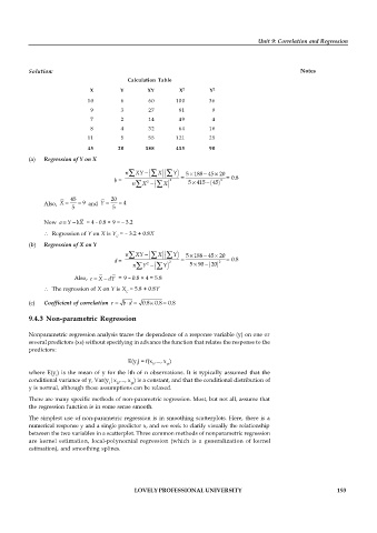
Calculation Table
X Y XY X 2 Y 2

10 6 60 100 36
9 3 27 81 9
7 2 14 49 4
8 4 32 64 16
11 5 55 121 25
45 20 188 415 90
(a) Regression of Y on X
nå XY - (å X )(å Y ) 5 188 45 20
-
´
´
b = nå X - (å X ) 2 = 5 415 - ( ) 2 = 0.8
´
45
2
Also, X = 45 = 9 and Y = 20 = 4
5 5
Now a Y= - bX = 4 - 0.8 × 9 = – 3.2

 Regression of Y on X is Y = – 3.2 + 0.8X
C
(b) Regression of X on Y
nå XY - (å X )(å Y ) 5 188 45 20
´
-
´
d = 2 = 2 = 0.8
nå Y - (å Y ) 5 90 - ( )
´
2
20
Also, c = X - dY = 9 – 0.8 × 4 = 5.8
 The regression of X on Y is X = 5.8 + 0.8Y
C
´
×
(c) Coefficient of correlation r = b d = 0.8 0.8 = 0.8
9.4.3 Non-parametric Regression
Nonparametric regression analysis traces the dependence of a response variable (y) on one or
several predictors (xs) without specifying in advance the function that relates the response to the
predictors:
E(y ) = f(x ,..., x )
i 1i pi
where E(y ) is the mean of y for the ith of n observations. It is typically assumed that the
i
conditional variance of y, Var(y |x ,..., x ) is a constant, and that the conditional distribution of
i 1i pi
y is normal, although these assumptions can be relaxed.
There are many specific methods of non-parametric regression. Most, but not all, assume that
the regression function is in some sense smooth.
The simplest use of non-parametric regression is in smoothing scatterplots. Here, there is a
numerical response y and a single predictor x, and we seek to clarify visually the relationship
between the two variables in a scatterplot. Three common methods of nonparametric regression
are kernel estimation, local-polynomial regression (which is a generalization of kernel
estimation), and smoothing splines.

LOVELY PROFESSIONAL UNIVERSITY 193