Page 231 - DMGT501_OPERATIONS_MANAGEMENT

Unit 8: Acceptance Sampling

occurs, because a lot with unacceptable quality was accepted. The symbol is commonly Notes
used for the Type II error and typical values range from 0.2 to 0.01.
5. Operating Characteristic (OC) Curve: This curve plots the probability of accepting the lot
(Y­axis) versus the lot fraction or percent defectives (X­axis). The OC curve is the primary
tool for displaying and investigating the properties of a LASP.
6. Average Outgoing Quality (AOQ): A common procedure, when sampling and testing is
non­destructive, is to 100% inspect rejected lots and replace all defectives with good units.
In this case, all rejected lots are made perfect and the only defects left are those in lots that
were accepted. AOQ’s refer to the long­term defect level for this combined LASP and 100%
inspection of rejected lots process. If all lots come in with a defect level of exactly p, and the
OC curve for the chosen (n,c) LASP indicates a probability pa of accepting such a lot, over
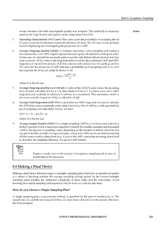
the long run the AOQ can easily be shown to be:

where N is the lot size.

7. Average Outgoing Quality Level (AOQL): A plot of the AOQ (Y­axis) versus the incoming
lot p (X­axis) will start at 0 for p = 0, and return to 0 for p = 1 (where every lot is 100%
inspected and rectified). In between, it will rise to a maximum. This maximum, which is

the worst possible long term AOQ, is called the AOQL.
8. Average Total Inspection (ATI): When rejected lots are 100% inspected, it is easy to calculate
the ATI if lots come consistently with a defect level of p. For a LASP (n,c) with a probability
pa of accepting a lot with defect level p, we have
ATI = n + (1 – pa) (N – n)
where N is the lot size.

9. Average Sample Number (ASN): For a single sampling LASP (n,c) we know each and every
lot has a sample of size n taken and inspected or tested. For double, multiple and sequential
LASP’s, the amount of sampling varies depending on the number of defects observed. For
any given double, multiple or sequential plan, a long term ASN can be calculated assuming
all lots come in with a defect level of p. A plot of the ASN, versus the incoming defect level
p, describes the sampling efficiency of a given LASP scheme.

Prepare a study note on the concept of acceptance sampling and its uses in
monitoring of the processes.

8.4 Making a Final Choice

Making a final choice between single or multiple sampling plans that have acceptable properties

is a matter of deciding whether the average sampling savings gained by the various multiple
sampling plans justifies the additional complexity of these plans and the uncertainty of not

knowing how much sampling and inspection will be done on a day­by­day basis.
How do you Choose a Single Sampling Plan?

A single sampling plan, as previously defined, is specified by the pair of numbers (n, c). The
sample size is n, and the lot is rejected if there are more than c defectives in the sample; otherwise
the lot is accepted.

LOVELY PROFESSIONAL UNIVERSITY 225