Page 230 - DMGT524_TOTAL_QUALITY_MANAGEMENT

Unit 14: Statistical Process Control

The probability distribution of a discrete random variable is a list of probabilities associated Notes
with each of its possible values. It is also sometimes called the probability function or the
probability mass function.

Example: Suppose a variable X can take the values 1, 2, 3, or 4.

The probabilities associated with each outcome are described by the following table:
Outcome 1 2 3 4
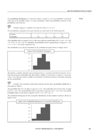
Probability 0.1 0.3 0.4 0.2

The probability that X is equal to 2 or 3 is the sum of the two probabilities: P(X = 2 or X = 3) = P(X
= 2) + P(X = 3) = 0.3 + 0.4 = 0.7. Similarly, the probability that X is greater than 1 is equal to 1 – P(X
= 1) = 1 – 0.1 = 0.9, by the complement rule.
This distribution may also be described by the probability histogram shown in Figure 14.15.

Figure 14.15: Probability Histogram
0.4

0.3

0.2

0.1

0.0
All random variables (discrete and continuous) have a cumulative distribution function. It is a
function giving the probability that the random variable X is less than or equal to x, for every
value x. For a discrete random variable, the cumulative distribution function is found by summing
up the probabilities.

Example: The cumulative distribution function for the above probability distribution is
calculated as follows:
The probability that X is less than or equal to 1 is 0.1, the probability that X is less than or equal
to 2 is 0.1 + 0.3 = 0.4, the probability that X is less than or equal to 3 is 0.1 + 0.3 + 0.4 = 0.8, and the
probability that X is less than or equal to 4 is 0.1 + 0.3 + 0.4 + 0.2 = 1.

The probability histogram for the cumulative distribution of this random variable is shown in
Figure 14.16.

Figure 14.16: Probability Histogram for Cumulative Distribution
1.0
0.8

0.6
0.4

0.2
0.0

LOVELY PROFESSIONAL UNIVERSITY 225