Page 121 - DCOM203_DMGT204_QUANTITATIVE_TECHNIQUES_I

Quantitative Techniques – I

Notes Solution.
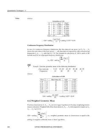
Calculation of GM
X f logX flogX
5 13 0.6990 9.0870
10 18 1.0000 18.0000
15 50 1.1761 58.8050
20 40 1.3010 52.0400
25 10 1.3979 13.9790
30 6 1.4771 8.8626
Total 137 160.7736

160.7736
GM = antilog = antilog 1.1735 = 14.91
137
Continuous Frequency Distribution

In case of a continuous frequency distribution, the class intervals are given. Let X , X , ......X
1 2 n
denote the mid-values of the first, second ...... nth class interval respectively with corresponding
frequencies f , f , ...... f , such that Sf = N. The formula for calculation of GM is same as the
1 2 n i
formula used for an ungrouped frequency distribution
f i log X i
i.e., GM = antilog N

Example: Calculate geometric mean of the following distribution:
Class Intervals : 5 -15 15 - 25 25 - 35 35 - 45 45 - 55
Frequencies : 10 22 25 20 8
Solution:
Calculation of GM
Class f Mid-Value (X) logX f logX
5-15 10 10 1.0000 10.0000
15-25 22 20 1.3010 28.6227
25-35 25 30 1.4771 36.9280
35-45 20 40 1.6020 32.0412
45-55 8 50 1.6990 13.5918
Total 85 121.1837
121.1837
GM = antilog = antilog 1.4257 = 26.65
85
6.6.2 Weighted Geometric Mean

If various observations, X , X , ......X , are not of equal importance in the data, weighted geometric
1 2 n
mean is calculated. Weighted GM of the observations X , X , ......X with respective weights as w ,
1 2 n 1
w ......w is given by :
2 n
w i log X i
GM = antilog , i.e., weighted geometric mean of observations is equal to the
w i
antilog of weighted arithmetic mean of their logarithms.

116 LOVELY PROFESSIONAL UNIVERSITY