Page 292 - DCOM203_DMGT204_QUANTITATIVE_TECHNIQUES_I

Unit 14: Poisson Probability Distribution

Notes
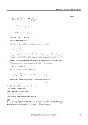
e m .m r m m r
r r 1 m e m
! r r 2 !
r 2 r 2

m 2 3 m 4 m 5
m e m m ....
2! 3!

2 3
2 m m m 2
m m e 1 m .... m m
2! 3!
Thus, Var(r) = m + m - m = m.
2
2
Also standard deviation m
2
3. The values of 1 : It can be shown that 3 = m and 4 = m + 3m .

2 m 2 1
3
1 3 3 m
2 m
Since m is a positive quantity, therefore, 1 is always positive and hence the Poisson
distribution is always positively skewed. We note that 0 as m , therefore the
distribution tends to become more and more symmetrical for large values of m.
Further, This result shows that the distribution becomes normal for large values of m.

4. Mode: As in binomial distribution, a Poisson variate r will be mode if
P r 1 P r P r 1

The inequality P r 1 P r can be written as

e m .m r 1 e m .m r m
1 r m .... (1)
r 1 ! r! r

Similarly, the inequality P r P r 1 can be shown to imply that
r m - 1 .... (2)

Combining (1) and (2), we can write m – 1 r m.
Case I. When m is not an integer
The integral part of m will be mode.

Case II. When m is an integer
The distribution is bimodal with values m and m – 1.

Example: The average number of customer arrivals per minute at a super bazaar is 2.
Find the probability that during one particular minute (1) exactly 3 customers will arrive, (2) at
the most two customers will arrive, (3) at least one customer will arrive.

LOVELY PROFESSIONAL UNIVERSITY 287