Page 296 - DCOM203_DMGT204_QUANTITATIVE_TECHNIQUES_I

Unit 14: Poisson Probability Distribution

14.1.3 Poisson Approximation to Binomial Notes

When n, the number of trials become large, the computation of probabilities by using the
binomial probability mass function becomes a cumbersome task. Usually, when n 20 and
p 0.05 , Poisson distribution can be used as an approximation to binomial with parameter m
= np.

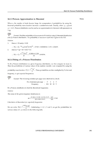
Example: Find the probability of 4 successes in 30 trials by using (1) binomial distribution
and (2) Poisson distribution. The probability of success in each trial is given to be 0.02.

Solution:
1. Here n = 30 and p = 0.02
30 4 26
P r 4 C 0.02 0.98 27405 0.00000016 0.59 0.00259.
4
2. Here m = np = 30 × 0.02 = 0.6
0.6 4
e 0.6 0.5488 0.1296
P r 4 0.00296.
4! 24
14.1.4 Fitting of a Poisson Distribution

To fit a Poisson distribution to a given frequency distribution, we first compute its mean m.
Then the probabilities of various values of the random variable r are computed by using the

e m .m r
probability mass function P r . These probabilities are then multiplied by N, the total
! r
frequency, to get expected frequencies.

Example: The following mistakes per page were observed in a book:
No. of mistakes per page : 0 1 2 3
Frequency : 211 90 19 5

Fit a Poisson distribution to find the theoretical frequencies.
Solution:
The mean of the given frequency distribution is

0×211+1×90 + 2×19 + 3×5 143
m = = = 0.44
211+90 +19 + 5 325
Calculation of theoretical (or expected) frequencies

e 0.44 0.44 r
We can write P r . Substituting r = 0, 1, 2 and 3, we get the probabilities for
r!
various values of r, as shown in the following table.

LOVELY PROFESSIONAL UNIVERSITY 291