Page 94 - DECO401_MICROECONOMIC_THEORY_ENGLISH

Unit-5: The Revealed Preference Theory of Demand

Notes
Fig. 5.3

L
P
Goods Y R B A

O
M Q S
Goods X

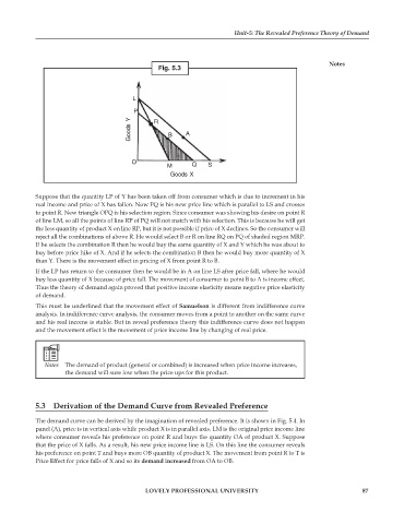
Suppose that the quantity LP of Y has been taken off from consumer which is due to increment in his
real income and price of X has fallen. Now PQ is his new price line which is parallel to LS and crosses
to point R. New triangle OPQ is his selection region. Since consumer was showing his desire on point R
of line LM, so all the points of line RP of PQ will not match with his selection. This is because he will get
the less quantity of product X on line RP, but it is not possible if price of X declines. So the consumer will
reject all the combinations of above R. He would select B or R on line RQ on PQ of shaded region MRP.
If he selects the combination R then he would buy the same quantity of X and Y which he was about to
buy before price hike of X. And if he selects the combination B then he would buy more quantity of X
than Y. There is the movement effect in pricing of X from point R to B.
If the LP has return to the consumer then he would be in A on line LS after price fall, where he would
buy less quantity of X because of price fall. The movement of consumer to point B to A is income effect.
Thus the theory of demand again proved that positive income elasticity means negative price elasticity
of demand.
This must be underlined that the movement effect of Samuelson is different from indifference curve
analysis. In indifference curve analysis, the consumer moves from a point to another on the same curve
and his real income is stable. But in reveal preference theory this indifference curve does not happen
and the movement effect is the movement of price income line by changing of real price.

The demand of product (general or combined) is increased when price income increases,
the demand will sure low when the price ups for this product.

5.3 Derivation of the Demand Curve from Revealed Preference

The demand curve can be derived by the imagination of revealed preference. It is shown in Fig. 5.4. In
panel (A), price is in vertical axis while product X is in parallel axis. LM is the original price income line
where consumer reveals his preference on point R and buys the quantity OA of product X. Suppose
that the price of X falls. As a result, his new price income line is LS. On this line the consumer reveals
his preference on point T and buys more OB quantity of product X. The movement from point R to T is
Price Effect for price falls of X and so its demand increased from OA to OB.

LOVELY PROFESSIONAL UNIVERSITY 87