Page 166 - DECO504_STATISTICAL_METHODS_IN_ECONOMICS_ENGLISH

Statistical Methods in Economics

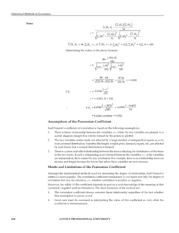
Notes ( )∑ ( fd fd ) ∑
∑ fd d – x y
y
x
N
r = ( fdx )∑ 2 ( fd ) ∑ 2
∑ fdx 2 – ∑ fdy 2 – y
N N
2
∑ fdd = 98, ∑ fd x = – 8, ∑ fd = – 8, ∑ fd x 2 = 122, ∑ fd y = 122, N = 100
y
y
x
Substituting the values in the above formula
( )–8 ( )–8
98 –
100
r = ( )–8 2 ( )–8 2
122 – 122 –
100 100

98–.64 97.36
= = = + 0.802
121.36 121.36 121.36

1– r 2
P.E. r = 0.6745
N
r = + 0.802, N = 100

( 1– ).802 2 1 – 0.6432
∴ P.E. = 0.6745 100 = 0.6745 10
r
= 0.6745 0.03568 = 0.024.
×
Assumptions of the Pearsonian Coefficient

Karl Pearson’s coefficient of correlation is based on the following assumptions:
1. There is linear relationship between the variables, i.e., when the two variables are plotted on a
scatter diagram straight line will be formed by the points so plotted.
2. The two variables under study are affected by a large number of independent causes so as to
form a normal distribution. Variables like height, weight, price, demand, supply, etc., are affected
by such forces that a normal distribution is formed.
3. There is a cause-and-effect relationship between the forces affecting the distribution of the items
in the two series. If such a relationship is not formed between the variables, i.e., if the variables
are independent, there cannot be any correlation. For example, there is no relationship between
income and height because the forces that affect these variables are not common.
Merits and Limitations of the Pearsonian Coefficient

Amongst the mathematical methods used for measuring the degree of relationship, Karl Pearson’s
method is most popular. The correlation coefficient summarises in one figure not only the degree of
correlation but also the direction, i.e., whether correlation is positive or negative.
However, the utility of this coefficient depends in part on a wide knowledge of the meaning of this
‘yardstick’, together with its limitations. The chief limitations of the method are:
1. The correlation coefficient always assumes linear relationship regardless of the fact whether
that assumption is correct or not.
2. Great care must be exercised in interpreting the value of this coefficient as very often the
coefficient is misinterpreted.

160 LOVELY PROFESSIONAL UNIVERSITY