Page 194 - DECO504_STATISTICAL_METHODS_IN_ECONOMICS_ENGLISH

Statistical Methods in Economics

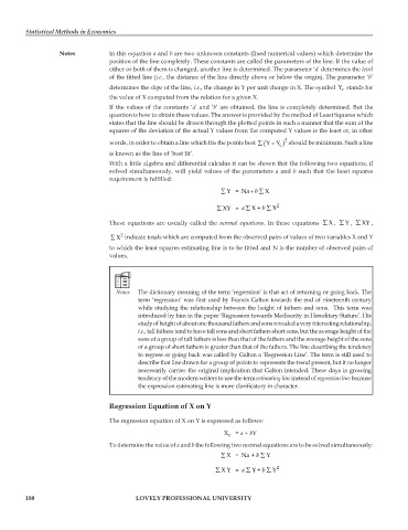
Notes In this equation a and b are two unknown constants (fixed numerical values) which determine the
position of the line completely. These constants are called the parameters of the line. If the value of
either or both of them is changed, another line is determined. The parameter ‘a’ determines the level
of the fitted line (i.e., the distance of the line directly above or below the origin). The parameter ‘b’
determines the slope of the line, i.e., the change in Y per unit change in X. The symbol Y stands for
c
the value of X computed from the relation for a given X.
If the values of the constants ‘a’ and ‘b’ are obtained, the line is completely determined. But the
question is how to obtain these values. The answer is provided by the method of Least Squares which
states that the line should be drawn through the plotted points in such a manner that the sum of the
squares of the deviation of the actual Y values from the computed Y values is the least or, in other
words, in order to obtain a line which fits the points best ( ∑ c )Y – Y 2 should be minimum. Such a line
is known as the line of ‘best fit’.
With a little algebra and differential calculus it can be shown that the following two equations, if
solved simultaneously, will yield values of the parameters a and b such that the least squares
requirement is fulfilled:
∑ Y = Nab
+∑ X
∑ XY = ∑ a ∑ X + b X 2

These equations are usually called the normal equations. In these equations ∑ X , ∑ Y , ∑ XY ,
2
∑ X indicate totals which are computed from the observed pairs of values of two variables X and Y
to which the least squares estimating line is to be fitted and N is the number of observed pairs of
values.

The dictionary meaning of the term ‘regression’ is that act of returning or going back. The
term ‘regression’ was first used by Francis Galton towards the end of nineteenth century
while studying the relationship between the height of fathers and sons. This term was
introduced by him in the paper ‘Regression towards Mediocrity in Hereditary Stature’. His
study of height of about one thousand fathers and sons revealed a very interesting relationship,
i.e., tall fathers tend to have tall sons and short fathers short sons, but the average height of the
sons of a group of tall fathers is less than that of the fathers and the average height of the sons
of a group of short fathers is greater than that of the fathers. The line describing the tendency
to regress or going back was called by Galton a ‘Regression Line’. The term is still used to
describe that line drawn for a group of points to represents the trend present, but it no longer
necessarily carries the original implication that Galton intended. These days is growing
tendency of the modern writers to use the term estimating line instead of regression line because
the expression estimating line is more clarificatory in character.

Regression Equation of X on Y

The regression equation of X on Y is expressed as follows:
X c = a + bY
To determine the value of a and b the following two normal equations are to be solved simultaneously:
a
∑ X = N + b ∑ Y
∑ X Y = ∑ a ∑ Y + b Y 2

188 LOVELY PROFESSIONAL UNIVERSITY