Page 295 - DMTH402_COMPLEX_ANALYSIS_AND_DIFFERENTIAL_GEOMETRY

Complex Analysis and Differential Geometry

Notes 23.5.3 A Parametrization of the Developable Surface

Once we have computed a curve c(t)  B that approximates the image points b(T ) well, the one-
i
parameter family E(t) determining the approximating developable surface D* is already given
by

E(t) : c (t) + c (t)x + c (t)y + c (t)z = 0.
2
3
4
1
The generating lines L(t) of D* are the intersection lines E(t)  E(t). We assume that there exist

two bounding planes H and H of the domain of interest in a way that all generating lines L(t)
2
1
intersect H and H in proper points. The intersection curves f (t) of L(t) and H , i = 1, 2 are
i
1
2
i
computed by
f (t) = E(t)  E(t)  H , i (10)

i
and the final point representation of D* is
x(t, u) = (1 – u)f (t) + uf (t). (11)
2
1
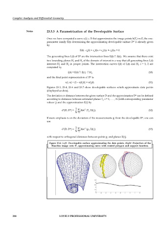
Figures 23.3, 23.4, 23.6 and 23.7 show developable surfaces which approximate data points
(displayed as dots).
The deviation or distance between the given surface D and the approximation D* can be defined
according to distances between estimated planes T , i = 1, . . . , N (with corresponding parameter
i
values t ) and the approximation E(t) by
i
1
2
d (D, D*) =  dist (T , E(t )). (12)
2
N i i i
If more emphasis is on the deviation of the measurements p from the developable D*, one can
i
use
1
d (D, D*) =  dist (p , E(t )). (13)
2
2
N i i i
with respect to orthogonal distances between points p and planes E(t ).
i
i
Figure 23.6: Left: Developable surface approximating the data points. Right: Projection of the
Blaschke image onto S , approximating curve with control polygon and support function.
2

288 LOVELY PROFESSIONAL UNIVERSITY