Page 297 - DMTH402_COMPLEX_ANALYSIS_AND_DIFFERENTIAL_GEOMETRY

Complex Analysis and Differential Geometry

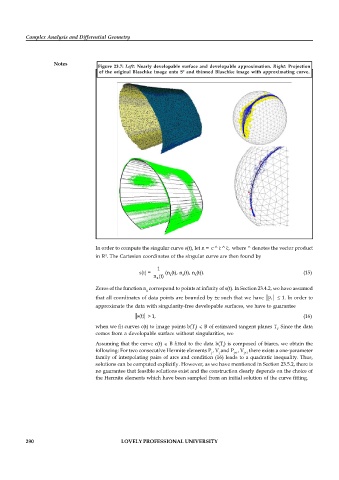
Notes Figure 23.7: Left: Nearly developable surface and developable approximation. Right: Projection
of the original Blaschke image onto S and thinned Blaschke image with approximating curve.
2

In order to compute the singular curve s(t), let n = c ^ c ^ c,  where ^ denotes the vector product

in  . The Cartesian coordinates of the singular curve are then found by
4
1
s(t) = (n (t), n (t), n (t)). (15)
n (t) 1 2 3
4
Zeros of the function n correspond to points at infinity of s(t). In Section 23.4.2, we have assumed
4
that all coordinates of data points are bounded by ±c such that we have p  1. In order to
i
approximate the data with singularity-free developable surfaces, we have to guarantee
s(t) > 1, (16)
when we fit curves c(t) to image points b(T )  B of estimated tangent planes T . Since the data
i
i
comes from a developable surface without singularities, we
Assuming that the curve c(t)  B fitted to the data b(T ) is composed of biarcs, we obtain the
i
following: For two consecutive Hermite elements P , V and P , V there exists a one-parameter
j+1
j
j+1
j
family of interpolating pairs of arcs and condition (16) leads to a quadratic inequality. Thus,
solutions can be computed explicitly. However, as we have mentioned in Section 23.5.2, there is
no guarantee that feasible solutions exist and the construction clearly depends on the choice of
the Hermite elements which have been sampled from an initial solution of the curve fitting.

290 LOVELY PROFESSIONAL UNIVERSITY