Page 181 - DMTH404_STATISTICS

Unit 13: Moment Generating Function - Continue

Notes
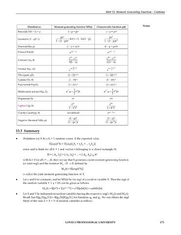
Distribution Moment-generating function MX(t) Characteristic function φ(t)
Bernoulli P(X = 1) = p 1 – p + pe t 1 – p + pe
it
pe t pe it


Geometric (1 – p) p for t  1 ln(1 p)
k–1

1 (1 p)e t 1 (1 p)e it



Binomial B(n, p) (1 – p + pe ) (1 – p + pe )
t n
it n
t it
Poisson Pois(λ) e  (e  1) e  (e  1)
tb
e  e ta e itb  e ita
Uniform U(a, b)
t(b a) it(b a)


1 2 2 1 2 2

Normal N(μ, σ2) t  t it –  t
2
e e
2
Chi-square χ2k (1 – 2t) –k/2 (1 – 2it) –k/2
–k
Gamma Γ(k, θ) (1 – t) (1 – it)
–k
Exponential Exp(λ) (1 – t ) (1 – it )
1 –1
1 –1
T
T
t
T
it
T
t
Multivariate normal N(μ, Σ) e   1 t  e   1 t 
t
2 2
Degenerate δa e e
ta
ita
e t e it
Laplace L(μ, b)
2 2
2 2

1 b t 1 b t

Cauchy Cauchy(μ, θ) not defined e it  –  |t|

(1 p) r (1 p) r

Negative Binomial NB(r, p)
t
it

(1 pe )r (1 pe )r


13.3 Summary
 Definition Let X be a K × 1 random vector. If the expected value
E[exp(t X) = E[exp(t X + t X + ... t X )]
T
1 1 2 2 K K
exists and is finite for all k × 1 real vectors t belonging to a closed rectangle H:
H = [–h , h ] × [–h , h ] × ... × [–h , h ]   K
1 1 2 2 K K
with hi > 0 for all i = ,...,K, then we say that X possesses a joint moment generating function
(or joint mgf) and the function M : H   defined by
X
M (t) = E[exp(t X)]
T
X
is called the joint moment generating function of X.
 Let a and b be constants, and let MX(t) be the mgf of a random variable X. Then the mgf of
the random variable Y = a + bX can be given as follows
at
tY
M (t) = E[e ] = E[e t(a + bX) ] = e E[e(bt)X] = eatMX(bt)
Y
 Let X and Y be independent random variables having the respective mgf’s M (t) and M (t).
X Y
Recall that E[g (X)g (Y)] = E[g (X)]E[g (Y)] for functions g and g . We can obtain the mgf
1 2 1 2 1 2
Mz(t) of the sum Z = X + Y of random variables as follows.
LOVELY PROFESSIONAL UNIVERSITY 173