Page 415 - DMTH404_STATISTICS

Unit 30: Method of Least Square

Solution. Notes

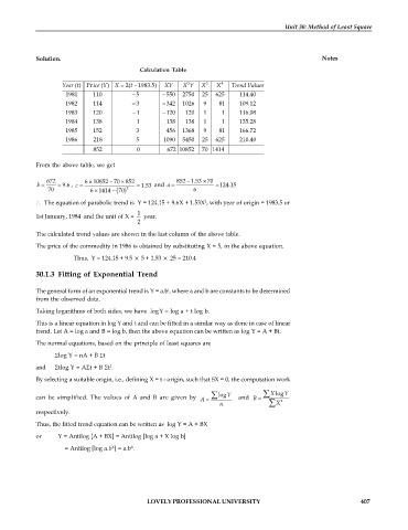
Calculation Table
2
Year ( ) Price ( ) X = 2(t  1983.5) XY X Y X 2 X 4 Trend Values
t
Y
1981 110  5  550 2750 25 625 114.40
1982 114  3  342 1026 9 81 109.12
1983 120  1  120 120 1 1 116.08
1984 138 1 138 138 1 1 135.28
1985 152 3 456 1368 9 81 166.72
1986 218 5 1090 5450 25 625 210.40
852 0 672 10852 70 1414
From the above table, we get

672 6 10852 70 852 852 1.53 70





b = = 9.6 , c = = 1.53 and a = = 124.15
70 6 1414  ( ) 2 6

70
 The equation of parabolic trend is Y = 124.15 + 9.6X + 1.53X , with year of origin = 1983.5 or
2
1
1st January, 1984 and the unit of X = year.
2
The calculated trend values are shown in the last column of the above table.
The price of the commodity in 1986 is obtained by substituting X = 5, in the above equation.
Thus, Y = 124.15 + 9.5  5 + 1.53  25 = 210.4
30.1.3 Fitting of Exponential Trend

t
The general form of an exponential trend is Y = a.b , where a and b are constants to be determined
from the observed data.
Taking logarithms of both sides, we have logY = log a + t log b.
This is a linear equation in log Y and t and can be fitted in a similar way as done in case of linear
trend. Let A = log a and B = log b, then the above equation can be written as log Y = A + Bt.

The normal equations, based on the principle of least squares are
log Y = nA + B t
and tlog Y = At + B t .
2
By selecting a suitable origin, i.e., defining X = t - origin, such that SX = 0, the computation work

can be simplified. The values of A and B are given by A = å logY and B = å X logY
2
n å X
respectively.
Thus, the fitted trend equation can be written as log Y = A + BX
or Y = Antilog [A + BX] = Antilog [log a + X log b]
= Antilog [log a.b ] = a.b .
X
X

LOVELY PROFESSIONAL UNIVERSITY 407