Page 109 - DMTH201_Basic Mathematics-1
P. 109
Basic Mathematics – I


                    Notes
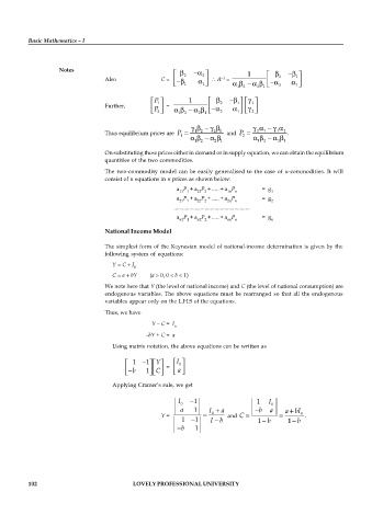
                                                            2     2             1         2     1
                                                                        –1
                                   Also              C =               A  =
                                                            1     1                       2     1
                                                                             1 2   2 1
                                                  P 1        1          2    1    1
                                   Further,            =
                                                  P
                                                   2      1 2    2 1    2    1    2

                                   Thus equilibrium prices are  P  1 2  2 1   and  P  2  1  1  2  .
                                                           1                   2
                                                               1 2    2 1          1 2    2 1
                                   On substituting these prices either in demand or in supply equation, we can obtain the equilibrium
                                   quantities of the two commodities.
                                   The two-commodity model can  be easily generalised to the  case  of  n-commodities. It will
                                   consist of n equations in n prices as shown below:
                                                          a P  + a P  + ..... + a P  = g
                                                          11 1  12 2      1n n          1
                                                          a P  + a P  + ..... + a P  = g
                                                          21 1  22 2      2n n          2
                                                         ......................................................
                                                          a P  + a P  + ..... + a P  = g
                                                          n1 1  n2 2      nn n          n
                                   National Income Model

                                   The simplest form of the Keynesian model of national-income determination is given by the
                                   following system of equations:
                                     Y = C + I
                                            0
                                     C = a + bY  (a > 0, 0 < b < 1)
                                   We note here that Y (the level of national income) and C (the level of national consumption) are
                                   endogenous variables. The above  equations must be rearranged  so that all the endogenous
                                   variables appear only on the L.H.S of the equations.
                                   Thus, we have
                                                  Y – C = I
                                                         0
                                                –bY + C = a
                                     Using matrix notation, the above equations can be written as

                                           1    1 Y       I 0
                                                       =
                                           b    1 C       a
                                     Applying Cramer’s rule, we get


                                                          I 0  1                   1   I 0
                                                           a   1    I   a           b  a    a bI
                                                     Y =             0    and C                  0  .
                                                           1   1    I  b            1 b      1 b
                                                           b   1


          102                               LOVELY PROFESSIONAL UNIVERSITY

