Page 261 - DCAP601_SIMULATION_AND_MODELING

Unit 13: Simulation Languages (I)

The obvious differences are in the three rates of decay of oscillation. Given the parameter values Notes
and initial conditions of Figure 13.9, the classic differential-equation and differential-delay-
equation models settle at equilibrium within four and 10 to 12 months, respectively, with an
overall human prevalence of 75%. Continuing out 10 years with the parameter values used in
Figure 13.9, an average over 25 runs shows overall human prevalence still oscillating slightly
(within 1%) around an overall human prevalence of 82%.
In the discrete-event model, immunity is considered a continuous process of change in the
probability that a previously exposed individual will block an infection when bitten by an
infectious mosquito, i.e., the parameter IM represents the rate of decay of immune resistance to
reinfection in an individual human. This operational view thereby incorporates the existence of
partial immunity to reinfection, an aspect of epidemiology difficult to represent in terms of the
discrete step transitions and flow rates of aggregate population-level models. That is, if adjacent
discrete compartments are “totally immune” and “totally susceptible,” and some quantity or
proportion is lost from one to the other over each interval of time, conventional differential-
equation models represent this loss as a rate of population flow between the two distinct states
rather than as a process of decay within each individual in a population.
These two views of immunity cannot be reconciled, but the models that embody them can be
compared by finding particular parameter values that relate an average duration of immunity
in an aggregate in the simulation model in its stationary state, to an equilibrium flow rate in the
differential-equation models. To do so requires the resolution of the full “age” distribution of
intervals since infection over all “immune” individuals in the simulation, relative to each
individual’s probability of becoming infected. The dynamics of the three systems away from
such fixed points of comparison may differ dramatically.
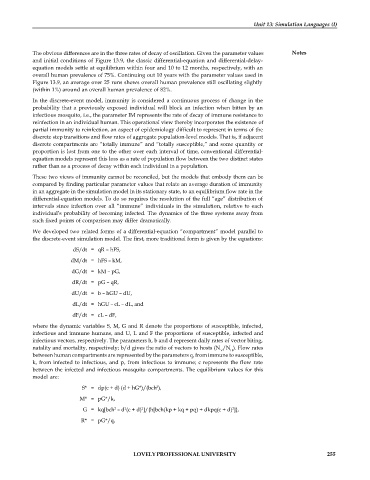
We developed two related forms of a differential-equation “compartment” model parallel to
the discrete-event simulation model. The first, more traditional form is given by the equations:
dS/dt = qR – hFS,
dM/dt = hFS – kM,

dG/dt = kM – pG,
dR/dt = pG – qR,
dU/dt = b – hGU – dU,
dL/dt = hGU – cL – dL, and
dF/dt = cL – dF,

where the dynamic variables S, M, G and R denote the proportions of susceptible, infected,
infectious and immune humans, and U, L and F the proportions of susceptible, infected and
infectious vectors, respectively. The parameters h, b and d represent daily rates of vector biting,
natality and mortality, respectively; b/d gives the ratio of vectors to hosts (N /N ). Flow rates
V H
between human compartments are represented by the parameters q, from immune to susceptible,
k, from infected to infectious, and p, from infectious to immune; c represents the flow rate
between the infected and infectious mosquito compartments. The equilibrium values for this
model are:

2
S* = dp(c + d) (d + hG*)/(bch ),
M* = pG*/k,
2
2
2
2
G = kq[bch – d (c + d) ]/{h[bch(kp + kq + pq) + dkpq(c + d) ]},
R* = pG*/q,

LOVELY PROFESSIONAL UNIVERSITY 255