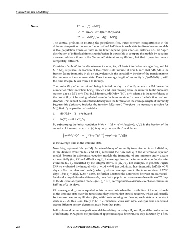
Page 262 - DCAP601_SIMULATION_AND_MODELING

Simulation and Modelling

Notes U* = b/(d + hG*)

L* = bhG*/[(c + d)(d + hG*)], and
F* = bchG*/[d(c + d)(d + hG*)].
The central problem in relating the population flow rates between compartments in the
differential-equation models to the individual half-lives in each state in discrete-event models
is that population transition rates in the latter depend upon infection histories, i.e., the “age”
distribution of individual times since infection. It is possible to compare the models by equating
average residence times in the “immune” state at an equilbrium, but their dynamics remain
completely different.
Consider a “cohort” in the discrete-event model, i.e., all hosts infected on a single day, and let
M = M(t) represent the fraction of that cohort still immune at time t, such that “dM/dt is the
fraction losing immunity in dt, or, equivalently, is the probability density of the transition from
the immune to the successor state. Then the average length of immunity is  (–dM/dt)dt, with
t
the time integral taken from 0 to infinity.
The probability of an individual being infected on day t is (1–e ), where q = IM, hence the
–qt
number of cohort members being infected and thus moving from the immune to the successor
–qt
state on day t is M(1–e ). That is, M decays as dM/dt = “M(1–e ), where q is the rate of decay of
–qt
the probability of becoming infected once in the immune state (i.e., once the infection has been
cleared). This cannot be substituted directly into the formula for the average length of immunity
because this derivative includes the function M(t) itself. Therefore it is necessary to solve for
M(t) first. By separation of variables:
–qt
1. dM/M = – (1 – e ) dt, and
2. In(M) = – (t + e )/q
–qt
–qt
By substituting the initial condition M(0) = 1, M = [e (1/q) ]/exp[t+(e /q)] is the fraction of the
x
cohort still immune, where exp(x) is synonymous with e , and hence:
q
 t (–dM / )dt =  t (1– e –qt )e (1/ )  /exp[t (e –qt / )]dt
q
dt
is the average time in the immune state.
Now let q represent this q(= IM), the rate of decay of immunity to reinfection in an individual,
s
in the discrete-event model, and let q represent the flow rate q in the differential-equation
c
model. Because in differential-equation models the immunity of any immune entity decays
exponentially (i.e., if G = 0, dR/dt = –q R), the average time in the immune state in the discrete-
c
event model, q , calculated by the integral above, is (ln2)/q . For example, to generate Figure
s c
13.9 we evaluated the integral with q = IM = 0.01 (an individual host immunity half-life of 70
s
days in the discrete-event model), which yields an average time in the immune state of 12.55
days. Thus q = ln(2)/12.55 = 0.055. To further illustrate the differences between an individual-
c
level and a population-level time scale, note that a population average residence time of 70 days
in the differential-equation models (i.e., q = 0.01) corresponds to a discrete-event-model immune
c
half-life of 2,166 days.
Of course q and q can be equated in this manner only when the distribution of the individuals
s c
in the immune state over the times since they entered that state is uniform, which will usually
be the case near an equilibrium (i.e., with hosts entering and leaving each state at a constant
daily rate). As this is not likely to be true elsewhere, even with identical equilibria one would
expect different system dynamics away from that point.
In this classic differential-equation model, translating the delays, D and D , and the host window
V H
of infectivity, WN, poses the problem of approximating a deterministic step function by a flow

256 LOVELY PROFESSIONAL UNIVERSITY