Page 50 - DCAP601_SIMULATION_AND_MODELING

Simulation and Modelling

Notes
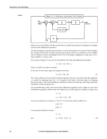
Figure 3.1: A Non-linear second-order Servo System

(Those of you not familiar with the control theory symbols may ignore the diagram and simply
start from the differential equation.)

This block diagram represents many natural as well as man-made servo systems. Some examples
are: beating of the heart, periodic opening and closing of flowers in response to the sunlight,
rate of variation of prices, squeaking of door with rusty hinges, dripping of a leaky tap, a neon-
lamp oscillator, to name a few.
The system of Figure 3.1 can also be described by the following differential equation:


 A(1 y )y By e i n
2
y 



where A and B are positive constants.
In the case of zero input signal, the equation becomes

 A(1 y )y By ...(1)
2
y 


This is the well-known Van der Pol non-linear equation. (It can be seen that when the amplitude
2
y is small, the damping term A(l – y ) is negative, but when y becomes large the damping
becomes positive. Thus small-amplitude oscillations will tend to build up, while large-amplitude
oscillations will be damped out.)
Let us simulate this system. The second-order differential equation can be written as a set of two
simultaneous equations of first order. We replace Eq. (1) with (using the variable y in place of y)
1
y  = y 2
1
2
y  = A(l – Y )Y – BY 1
2
1
2
To be more specific let constants A = 0.1, B = l.0 and let the initial conditions be
y (0) = l.0
1
y (0) = 0.
2
Our equations therefore become
y  = y
1 2
2
and y  = 0.1(l – Y )Y – Y ... (2)
2 1 2 1

44 LOVELY PROFESSIONAL UNIVERSITY