Page 53 - DCAP601_SIMULATION_AND_MODELING

Unit 3: Simulation of Continuous System (II)

Notes
!
Caution To better administer potential changes to reservoir operations given worries or
changes in circumstances, it is helpful to build up a calibrated simulation model of the reservoir

Let us consider the following proposal for constructing a dam across a river to create a reservoir.
The reservoir is to be constructed at a specified site. The curve of the projected demand for the
water from the reservoir has been determined (from the expected growth pattern and the seasonal
fluctuations). The input to the reservoir is from the river inflow and from the rainfall directly
over the reservoir. The output consists of the seepage and evaporation losses, in addition to the
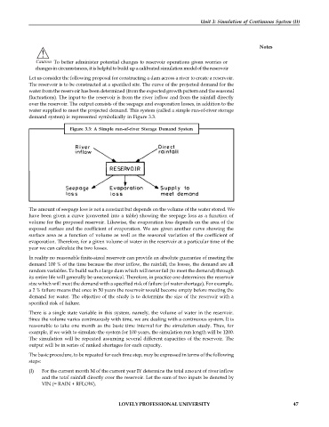
water supplied to meet the projected demand. This system (called a simple run-of-river storage
demand system) is represented symbolically in Figure 3.3.

Figure 3.3: A Simple run-of-river Storage Demand System

The amount of seepage loss is not a constant but depends on the volume of the water stored. We
have been given a curve (converted into a table) showing the seepage loss as a function of
volume for the proposed reservoir. Likewise, the evaporation loss depends on the area of the
exposed surface and the coefficient of evaporation. We are given another curve showing the
surface area as a function of volume as well as the seasonal variation of the coefficient of
evaporation. Therefore, for a given volume of water in the reservoir at a particular time of the
year we can calculate the two losses.
In reality no reasonable finite-sized reservoir can provide an absolute guarantee of meeting the
demand 100 % of the time because the river inflow, the rainfall, the losses, the demand are all
random variables. To build such a large dam which will never fail (to meet the demand) through
its entire life will generally be uneconomical. Therefore, in practice one determines the reservoir
size which will meet the demand with a specified risk of failure (of water shortage). For example,
a 2 % failure means that once in 50 years the reservoir would become empty before meeting the
demand for water. The objective of the study is to determine the size of the reservoir with a
specified risk of failure.
There is a single state variable in this system, namely, the volume of water in the reservoir.
Since the volume varies continuously with time, we are dealing with a continuous system. It is
reasonable to take one month as the basic time interval for the simulation study. Thus, for
example, if we wish to simulate the system for 100 years, the simulation run length will be 1200.
The simulation will be repeated assuming several different capacities of the reservoir. The
output will be in series of ranked shortages for each capacity.
The basic procedure, to be repeated for each time step, may be expressed in terms of the following
steps:

(l) For the current month M of the current year IY determine the total amount of river inflow
and the total rainfall directly over the reservoir. Let the sum of two inputs be denoted by
VIN (= RAIN + RFLOW).

LOVELY PROFESSIONAL UNIVERSITY 47