Page 55 - DCAP601_SIMULATION_AND_MODELING

Unit 3: Simulation of Continuous System (II)

20 PRINT, FLOW, RAIN, TLOSS, SHORT, SPILL, VOL Notes
30 CONTINUE
STOP
END

Subroutines

The foregoing program contains five subroutines requiring data about the riverflow, rainfall
and the demand as a function of time; the seepage loss as a function of water stored in the
reservoir; and the evaporation loss as a function of the volume (and hence the exposed surface)
and the particular month of the year. The long sequence of data for river inflow and the rainfall
could either be obtained from historical records or generated using suitable pseudorandom
number generators. Similarly we can design the other subroutines, from an intimate knowledge
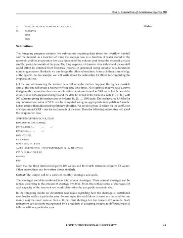
of the system. As an example, we will write down the subroutine EVPRSN, for computing the
evaporation loss.
Let the unit of measuring the volume be a million cubic meters. Suppose the highest possible
dam at this site will create a reservoir of capacity 1000 units. Also suppose that we have a curve
that gives the exposed surface area as a function of volume from 0 to 1000 units. Let the x-axis be
divided into 100 equispaced ranges; and the data be stored in the form of a table (SURTBL) with
100 columns giving the surface area at volume 10, 20, ... , 1000 units. The surface area SAREA for
any intermediate value of VOL can be computed using an appropriate interpolation formula.
Let us assume that a linear interpolation will suffice. We are also given 12 values for the coefficient
of evaporation COEF – one for each month of the year. Then the following subroutine will yield
the evaporation loss.

SUBROUTINE EVPRSN (M, VOL, EVAP)
REAL SURTBL (100), COEF(12)
DATA SURTBL /..., ..., .../
DATA COEF /..., ..., .../
IVOL = VOL/10.
RVOL = IVOL
FRAC = VOL/10. – R VOL
SAREA = SURTBL (IVOL) + FRAC*(SURTBL(IVOL+l) – SURTBL(IVOL))
EVAP = SAREA * COEF (M)
RETURN
END
Note that the third statement requires 100 values and the fourth statement requires 12 values.
Other subroutines can be written down similarly.
Output: The output will be a series of monthly shortages and spills.
The shortages could be combined into total annual shortages. These annual shortages can be
ranked according to the amount of shortage involved. From this ranked series of shortages for
each capacity of the reservoir we would determine the acceptable reservoir size.
In the foregoing model no distinction was made regarding how the shortage is distributed
month-wise within a particular year. For example, the total failure to meet any demand for one
month may be more serious than a 10 per cent shortage for ten consecutive months. Such
refinement can be easily incorporated by a procedure of assigning weights to different types of
failures within a particular year.

LOVELY PROFESSIONAL UNIVERSITY 49