Page 68 - DCAP603_DATAWARE_HOUSING_AND_DATAMINING

Data Warehousing and Data Mining

notes classifiers. Naive Bayesian classifiers assume that the effect of an attribute value on a given class
is independent of the values of the other attributes. This assumption is called class conditional
independence. It is made to simplify the computations involved, and in this sense, is considered
“naive”. Bayesian belief networks are graphical models, which unlike naive Bayesian classifiers,
allow the representation of dependencies among subsets of attributes.
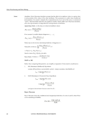
Apply Bayes Rule: c is the class, {v} observed attribute values:
({ }| ) ( ) c
P v c P
P c v
( |{ }) =
({ })
P v
If we assume k possible disjoint diagnoses, c , …, c
1 K
c
v
P
P ({ } ({ }| c )
( P c k |{ }) = k P ({ }) k
v
v
P({v}) may not be known, but total probability of diagnoses is 1
c
P
v
k
P({v}) (the evidence): Â P ({ } ({ }| c k ) = 1
({ })
k P v
⇒ P({v}) = S |P(c ) P({v}|c |
k k k
Need to know P(c ), P({v}|c ) for all k
k
k
Bayes Rules:
Map vs. ML
Rather than computing full posterior, can simplify computation if interested in classification:

1. ML (Maximum Likelihood) Hypothesis
assume all hypotheses equiprobable a priori – simply maximize data likelihood:
v
c
c = argmax ({ }| )
P
ML
Œ
c C
2. MAP (Maximum A Posteriori) Class Hypothesis
v
P
c
c MAP = argmax ( |{ })
Œ
c C
P ({ } | ( ))
c
v
c
P
= argmax
v
Œ
c C P ({ })
can ignore denominator because same for all c
Bayes theorem
Bayes’ theorem relates the conditional and marginal probabilities of events A and B, where B has
a non-vanishing probability:
A
B
A
P
P ( | ) ( )
B
P ( | ) = .
A
B
P ( )
62 LoveLy professionaL university