Page 71 - DCAP603_DATAWARE_HOUSING_AND_DATAMINING

Unit 4: Data Mining Classification

notes

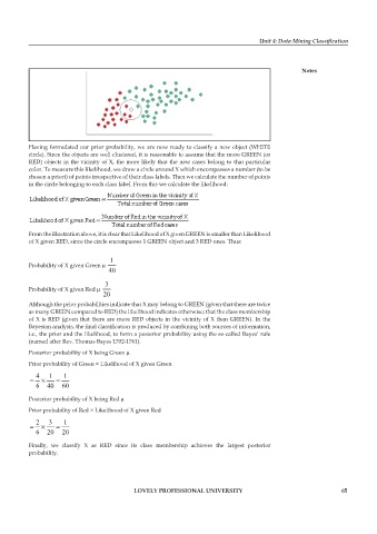
Having formulated our prior probability, we are now ready to classify a new object (WHITE
circle). Since the objects are well clustered, it is reasonable to assume that the more GREEN (or
RED) objects in the vicinity of X, the more likely that the new cases belong to that particular
color. To measure this likelihood, we draw a circle around X which encompasses a number (to be
chosen a priori) of points irrespective of their class labels. Then we calculate the number of points
in the circle belonging to each class label. From this we calculate the likelihood:

From the illustration above, it is clear that Likelihood of X given GREEN is smaller than Likelihood
of X given RED, since the circle encompasses 1 GREEN object and 3 RED ones. Thus:

1
Probability of X given Green µ
40
3
Probability of X given Red µ
20
Although the prior probabilities indicate that X may belong to GREEN (given that there are twice
as many GREEN compared to RED) the likelihood indicates otherwise; that the class membership
of X is RED (given that there are more RED objects in the vicinity of X than GREEN). In the
Bayesian analysis, the final classification is produced by combining both sources of information,
i.e., the prior and the likelihood, to form a posterior probability using the so-called Bayes’ rule
(named after Rev. Thomas Bayes 1702-1761).

Posterior probability of X being Green µ
Prior probability of Green × Likelihood of X given Green
4 1 1
= ¥ =
6 40 60

Posterior probability of X being Red µ
Prior probability of Red × Likelihood of X given Red
2 3 1
= ¥ =
6 20 20

Finally, we classify X as RED since its class membership achieves the largest posterior
probability.

LoveLy professionaL university 65