Page 69 - DCAP603_DATAWARE_HOUSING_AND_DATAMINING
P. 69
Unit 4: Data Mining Classification


          Each term in Bayes’ theorem has a conventional name:                                  notes
          1.   P(A) is the prior probability or marginal probability of A. It is “prior” in the sense that it
               does not take into account any information about B.
          2.   P(A|B) is the conditional probability of A, given B. It is also called the posterior probability
               because it is derived from or depends upon the specified value of B.

          3.   P(B|A) is the conditional probability of B given A.
          4.   P(B) is the prior or marginal probability of B, and acts as a normalizing constant.
          Intuitively, Bayes’ theorem in this form describes the way in which one’s beliefs about observing
          ‘A’ are updated by having observed ‘B’.

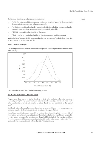
          Bayes Theorem: Example

          Use training examples to estimate class-conditional probability density functions for white-blood
          cell count (W)

                            0.4
                           0.35

                            0.3

                           0.25

                         P(W/D i )   0.2

                           0.15
                            0.1

                           0.05

                             0     20      25      30      35      40      45      50      55      60


                                          White blood cell count (W)

          Could use these to select maximum likelihood hypothesis.

          4.4 Naive Bayesian Classification


          Suppose  your  data  consist  of  fruits,  described  by  their  color  and  shape.  Bayesian  classifiers
          operate by saying “If you see a fruit that is red and round, which type of fruit is it most likely
          to be, based on the observed data sample? In future, classify red and round fruit as that type of
          fruit.”
          A difficulty arises when you have more than a few variables and classes - you would require an
          enormous number of observations (records) to estimate these probabilities.
          Naive  Bayes  classification  gets  around  this  problem  by  not  requiring  that  you  have  lots  of
          observations for each possible combination of the variables. Rather, the variables are assumed to
          be independent of one another and, therefore the probability that a fruit that is red, round, firm,
          3” in diameter, etc. will be an apple can be calculated from the independent probabilities that a
          fruit is red, that it is round, that it is firm, that it is 3” in diameter, etc.


                                           LoveLy professionaL university                                    63

