Page 102 - DMGT202_COST_AND_MANAGEMENT_ACCOUNTING

Unit 6: Marginal Costing and Absorption Costing

6.7 Methods Decisions Involving Alternative Choices Notes

The break even analysis can be performed by the following two methods:
1. Break Even Charts
2. Algebraic Method.

6.7.1 Break Even Chart

The difference between Price and Average Variable Cost (P – AVC) is defined as ‘profi t
contribution’. That is, revenue on the sale of a unit of output after variable costs are covered

represents a contribution toward profit. At low rates of output, the firm may be losing money

because fixed costs have not yet been covered by the profit contribution. Thus, at these low rates

of output, profit contribution is used to cover fixed costs. After fixed costs are covered, the fi rm

will be earning a profi t.
A manager may want to know the output rate necessary to cover all fixed costs and to earn a

“required” profit of R. Assume that both price and variable cost per unit of output (AVC) are
constant. Profit is equal to total revenue (P.Q.) less the sum of Total Variable Costs (Q.TVC) and

fixed costs. Thus
Π = PQ – [(Q. AVC) + FC]
R
Π = TR – TC
R
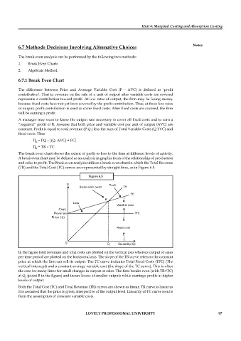
The break even chart shows the extent of profit or loss to the firm at different levels of activity.

A break even chart may be defined as an analysis in graphic form of the relationship of production
and sales to profit. The Break even analysis utilises a break even chart in which the Total Revenue

(TR) and the Total Cost (TC) curves are represented by straight lines, as in Figure 6.5.
Figure 6.5

`

In the figure total revenues and total costs are plotted on the vertical axis whereas output or sales

per time period are plotted on the horizontal axis. The slope of the TR curve refers to the constant

price at which the firm can sell its output. The TC curve indicates Total Fixed Costs (TFC) (The
vertical intercept) and a constant average variable cost (the slope of the TC curve). This is often
the case for many firms for small changes in output or sales. The firm breaks even (with TR=TC)

at Q (point B in the fi gure) and incurs losses at smaller outputs while earnings profi ts at higher
1
levels of output.
Both the Total Cost (TC) and Total Revenue (TR) curves are shown as linear. TR curve is linear as
it is assumed that the price is given, irrespective of the output level. Linearity of TC curve results
from the assumption of constant variable costs.

LOVELY PROFESSIONAL UNIVERSITY 97