Page 115 - DCOM303_DMGT504_OPERATION_RESEARCH
P. 115
Operations Research


                    Notes
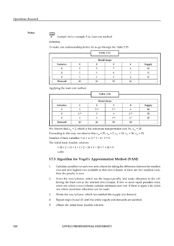
                                        Example: Solve example 5 by least cost method.
                                   Solution:

                                   To make our understanding better, let us go through the Table 5.15.
                                                                     Table  5.15

                                                                    Retail shops
                                        Factories      1           2          3           4         Supply
                                           1           3           5          7           6           50
                                           2           2           5          8           2           75
                                           3           3           6          9           2           25
                                        Demand         20         20          50          60

                                   Applying the least cost method-

                                                                     Table  5.16

                                                                    Retail shops
                                        Factories      1           2          3           4         Supply
                                           1           3          5           7           6           50
                                                                               30
                                                                   20
                                           2           2           5          8          2            75
                                                                                           55
                                                        20
                                                                               20
                                           3           3           6          9           2    5      25
                                        Demand         20         20          50          60

                                   We observe that c  = 2, which is the minimum transportation cost. So, x  = 20.
                                                 21                                          21
                                   Proceeding in this way, we observe that x  = 55, x  = 5, x  = 20, x  = 30, x  = 20.
                                                                    24     34    12     13    33
                                   Number of basic variables = m + n –1 = 3 + 4 – 1 = 6.
                                   The initial basic feasible solution:
                                        = 20 × 2 + 55 × 2 + 5 × 2 + 20 × 5 + 30 × 7 + 20 × 9
                                        = 650.

                                   5.7.3 Algorithm for Vogel’s Approximation Method (VAM)

                                   1.  Calculate penalties for each row and column by taking the difference between the smallest
                                       cost and next highest cost available in that row/column. If there are two smallest costs,
                                       then the penalty is zero.
                                   2.  Select the row/column, which has the largest penalty and  make allocation in the cell
                                       having the least cost in the selected row/column. If two or more equal penalties exist,
                                       select one where a row/column contains minimum unit cost. If there is again a tie, select
                                       one where maximum allocation can be made.

                                   3.  Delete the row/column, which has satisfied the supply and demand.
                                   4.  Repeat steps (1) and (2) until the entire supply and demands are satisfied.
                                   5.  Obtain the initial basic feasible solution.


          110                               LOVELY PROFESSIONAL UNIVERSITY

